HandyCNV Vignette
Jinghang ZHOU, Thomas Lopdell, Liyuan Liu, Dorian Garrick, Yuangang Shi
September 24, 2021
HandyCNV.RmdIntroduction
This package was originally designed for the Post-analysis of CNV results inferred from PennCNV and CNVPartition (GenomeStudio). However, it has now been expanded to accept input files in standard formats for a wider range of applications. Our motivation is to provide a standard, reproducible and time-saving pipeline for the post-analysis of CNVs and ROHs detected from SNP genotyping data for the majority of diploid Species. The functions provided in this package can be categorised into five sections: Conversion, Summary, Annotation, Comparison and Visualization. The most useful features provided are: integrating summarized results, generating lists of CNVR, annotating the results with known gene positions, plotting CNVR distribution maps, and producing customised visualisations of CNVs and ROHs with gene and other related information on one plot. This package also supports a range of customisations, including the colour, size of high resolution figures, and output folder, avoiding conflict between the results of different runs. Running through all functions detailed in the vignette could help us to identify and explore the most interesting genomic regions more easily. In the following sections, we will present how to use the functions provided in this package to solve these problems.
Installation and Prerequisites
First, to run this package, we need to make sure that R (Version >= 3.5.2) is installed in your computer (R download link: https://www.r-project.org/). Once R is installed, the ‘HandyCNV’ package can be installed from Github repository by running the following script. If you rarely used R, it may take more time to install the ‘HandyCNV’ for the first time.
#install.packages("remotes")
#library(remotes)
#install_github(repo = "JH-Zhou/HandyCNV")
Then, we need to load the ‘HandyCNV’ package in order to run the following examples. This can be done using the library function as shown below.
library(HandyCNV)To start playing with this package, we first need to prepare at least one CNV result list. With only CNV results as an input file, we can explore the functions from section 1 to section 10 as below. But to get more interesting and potentially valuable results, we will have to prepare additional input files, including the map file and signal intensity file for the SNP chip used to generate the CNV list, the pedigree of the samples, and Plink format (bed, bim and fam) genotype files. Many of these files are already required during CNV discovery, and by generating them early in the pipeline, you will find that the rest of workflow will be much easier and faster. We will be introducing how to prepare each of the input files in the relevant chunks below.
Demo data
We have provided some internal demo data, which should installed with package, in order to demonstrate how to use this package. We can access the demo data using the built-in R function system.file (see examples below). In the demo data, the first CNV results file is the default output from PennCNV with the ARS-UCD 1.2 (ARS) cattle reference genome. The second CNV results file contains the default output from CNVPartition with UMD 3.1 (UMD) cattle reference genome, and the third CNV list is an example of a standard input file that could be prepared from CNV results inferred by other tools.
Note: If you prefer not to test with this demo data, just skip this step to section 1 and use your own data instead.
cnv_penn_ars <- system.file("extdata", "Demo_data/cnv_results/ARS_PennCNV_WGC.goodcnv", package = "HandyCNV")
cnv_part_umd <- system.file("extdata", "Demo_data/cnv_results/UMD_CNVPartition.txt", package = "HandyCNV")
cnv_other_umd <- system.file("extdata", "Demo_data/cnv_results/UMD_Standard_CNV.txt", package = "HandyCNV")
Setting up a working directory
To start the analysis, let’s first set up the working directory. This will help ensure that all results will be saved in the same directory.
setwd(dir = "C:/Users/handy_test") #remember to replace the path with your own What issues can this package solve?
As above we mentioned, the functions in the package have been categorised into five sections: Conversion, Summary, Annotation, Comparison and Visualization.
Functions in the Conversion section can, for example, be used to convert coordinates between the default and target mapfiles provided by users; this would be useful if we are detecting CNVs with two different reference genomes. The converted map files can be output in formats suitable for use in Plink, PennCNV and our package ‘HandyCNV’. It is also possible to convert coordinates for intervals (CNV, CNVR, QTL et al) between the defaults and target maps, which might useful when comparing the results to those of other researchers. Functions included in the Summarization section allow the formatting and plotting of outputs, such as producing detailed summaries of CNVs and ROHs, making CNV summary plots, generating CNV regions (CNVRs), and plotting CNVR distribution maps.
The Annotation section allows the downloading of reference gene lists from the UCSC website, enabling the annotation of CNV, CNVR, ROH or other intervals with gene locations. The Comparison section facilitates the comparison of CNVs, CNVRs, Gene Frequent Lists and any other intervals. The highlight of this section is that comparison of CNVs and CNVRs will produce reports detailing comparison results on both individual and population levels, and all comparison results are relative to both input files. Finally, the Visualization section contains functions to support customised CNV and ROH plotting by chromosome, specific sample, regions of interest, or target genes (plotting by gene is not yet available for ROH). It is also possible to annotate the plots with other information, such as gene locations, log R ratio, B Allele Frequency, SNP genotype, LD or the source of CNVs. These functions can also plot genes separately from reference gene lists, which might useful for comparing outputs with plots from other studies.
Now, let’s start exploring the functions in HandyCNV.
1. How do we prepare the standard cnv input file for HandyCNV and get a quick summary?
We can use cnv_clean function to convert cnv results to standard format. This function will also produce a brief summary of CNV results. First, let’s format the sample CNV results from PennCNV. Note:
- When formatting results in PennCNV format, the corresponding CNV input argument is ‘penncnv’.
- Default PennCNV results in Sample ID columns usually have the file path ahead the Sample ID. For example with the file “/home/zjhang027/C/final_403_penncnv/201094560082_R03C01.txt”, the pattern ‘cnv/’ before the sample ID is unique, so we can take it as the separator using the argument
penn_id_sep = "cnv/"to extract the wanted sample ID.
cnv_penn_ars <- cnv_clean(penncnv = cnv_penn_ars, #replace input file when running your own data
                 penn_id_sep = "cnv/", #take the unique pattern as a separator to extract the sample ID
                 drop_length = 5, # the maximum CNV length threshold (in Mb); CNVs larger than this value will be deleted
                 folder = "cnv_clean") #create a new folder to save results
#> There are 382 individuals with 5215 CNVs in total.
#> The average number of CNVs present per individual is 13.65
#> Basic summary stats by CNV type:
#> # A tibble: 4 x 5
#>   CNV_Value     N `Average Length` `Min Length` `Max Length`
#>   <chr>     <int>            <dbl>        <dbl>        <dbl>
#> 1 0           146            65930         9932       343728
#> 2 1          2446           129081         1181      2822505
#> 3 3          2450           257261         6735      3651356
#> 4 4           173           687524        17406      4917181
Next, let’s format a second set of CNV results, this time produced using CNVPartition. Note: The corresponding input argument is cnvpartition for CNV result from CNVPartition.
cnv_part_umd <- cnv_clean(cnvpartition = cnv_part_umd, #when running your own data, set this argument by 'cnvpartition = "localpath/file"'
                 drop_length = 5, #the maximum CNV length threshold (in Mb); CNVs larger than this value will be deleted
                 folder = "cnv_clean")
#> There are 365 individuals with 1239 CNVs in total.
#> The average number of CNV on each Individual is 3.39
#> Basic summary stats by CNV type:
#> # A tibble: 4 x 5
#>   CNV_Value     N `Average Length` `Min Length` `Max Length`
#>       <int> <int>            <dbl>        <dbl>        <dbl>
#> 1         0   754           148699         4510      1204452
#> 2         1    59           375120        14229      3440849
#> 3         3   409           840778         4908      4867751
#> 4         4    17           634036        58524      2336934
If the CNV results were not produced by PennCNV or CNVPartition, we need to arrange the CNV results into the standard format, then use the standard_cnv argument instead. The standard CNV input list should include the following columns (in order): Sample_ID, Chr, Start, End and CNV_Value.
library(knitr)
kable(data.frame(Sample_ID = c("201977910077_R05C01", "201094560084_R06C02", "201094560084_R06C02", "201094560067_R08C02", "201094560067_R08C02"),
           Chr = c(6, 7, 7, 4, 4),
           Start = c(9087392, 28583247, 37214745, 6248795, 66567441),
           End = c(9250902, 28621254, 37238472, 6425277, 66830563),
CNV_Value = c(1, 3, 1, 3, 3)))| Sample_ID | Chr | Start | End | CNV_Value |
|---|---|---|---|---|
| 201977910077_R05C01 | 6 | 9087392 | 9250902 | 1 |
| 201094560084_R06C02 | 7 | 28583247 | 28621254 | 3 |
| 201094560084_R06C02 | 7 | 37214745 | 37238472 | 1 |
| 201094560067_R08C02 | 4 | 6248795 | 6425277 | 3 |
| 201094560067_R08C02 | 4 | 66567441 | 66830563 | 3 |
Let’s now run cnv_clean on the third Standard CNV input file. Note that we are using the argument standard_cnv for the third CNV result.
cnv_standard <- cnv_clean(standard_cnv = cnv_other_umd, #when running your own data, set this argument by 'standard_cnv = "localpath/file"'
                 drop_length = 5, #the maximum CNV length threshold (in Mb); CNVs larger than this value will be deleted
                 folder = "cnv_clean")
#> There are 382 individuals with 4534 CNVs in total.
#> The average number of CNV per individual is 11.87
#> Basic summary stats by CNV type:
#> # A tibble: 4 x 5
#>   CNV_Value     N `Average Length` `Min Length` `Max Length`
#>       <int> <int>            <dbl>        <dbl>        <dbl>
#> 1         0    77            60964         9932       343900
#> 2         1  2187           138295            1      2843668
#> 3         3  2115           258623            1      3933681
#> 4         4   155           779553        17392      4869255
2 How do we visualise CNVs?
The cnv_visual function supports visualising CNVs by chromosome, single sample, regions of interest, and target genes.
2.1 How do we have a quick overview of all CNVs on each chromosome?
Once we got the standard clean_cnv result, we can use the cnv_visual function to plot all CNVs, to have a quick look if there are any notable patterns in CNV results.
First, let’s visualise the whole PennCNV dataset across all chromosomes:
cnv_visual(clean_cnv = cnv_penn_ars, #standard file was generated by 'cnv_clean' function in section 1
           max_chr = 29, #select how many chromosomes to plot
           width_1 = 20, #optional,adjust the width of final plot
           height_1 =12, #optional,adjust the height of final plot
           folder = "cnv_visual_all_penn")
#> Input data passed requirment check...
#> [1] "Plotting the CNVs on Chromosome 1"
#> [1] "Plotting the CNVs on Chromosome 2"
#> [1] "Plotting the CNVs on Chromosome 3"
#> [1] "Plotting the CNVs on Chromosome 4"
#> [1] "Plotting the CNVs on Chromosome 5"
#> [1] "Plotting the CNVs on Chromosome 6"
#> [1] "Plotting the CNVs on Chromosome 7"
#> [1] "Plotting the CNVs on Chromosome 8"
#> [1] "Plotting the CNVs on Chromosome 9"
#> [1] "Plotting the CNVs on Chromosome 10"
#> [1] "Plotting the CNVs on Chromosome 11"
#> [1] "Plotting the CNVs on Chromosome 12"
#> [1] "Plotting the CNVs on Chromosome 13"
#> [1] "Plotting the CNVs on Chromosome 14"
#> [1] "Plotting the CNVs on Chromosome 15"
#> [1] "Plotting the CNVs on Chromosome 16"
#> [1] "Plotting the CNVs on Chromosome 17"
#> [1] "Plotting the CNVs on Chromosome 18"
#> [1] "Plotting the CNVs on Chromosome 19"
#> [1] "Plotting the CNVs on Chromosome 20"
#> [1] "Plotting the CNVs on Chromosome 21"
#> [1] "Plotting the CNVs on Chromosome 22"
#> [1] "Plotting the CNVs on Chromosome 23"
#> [1] "Plotting the CNVs on Chromosome 24"
#> [1] "Plotting the CNVs on Chromosome 25"
#> [1] "Plotting the CNVs on Chromosome 26"
#> [1] "Plotting the CNVs on Chromosome 27"
#> [1] "Plotting the CNVs on Chromosome 28"
#> [1] "Plotting the CNVs on Chromosome 29"
#> Task done.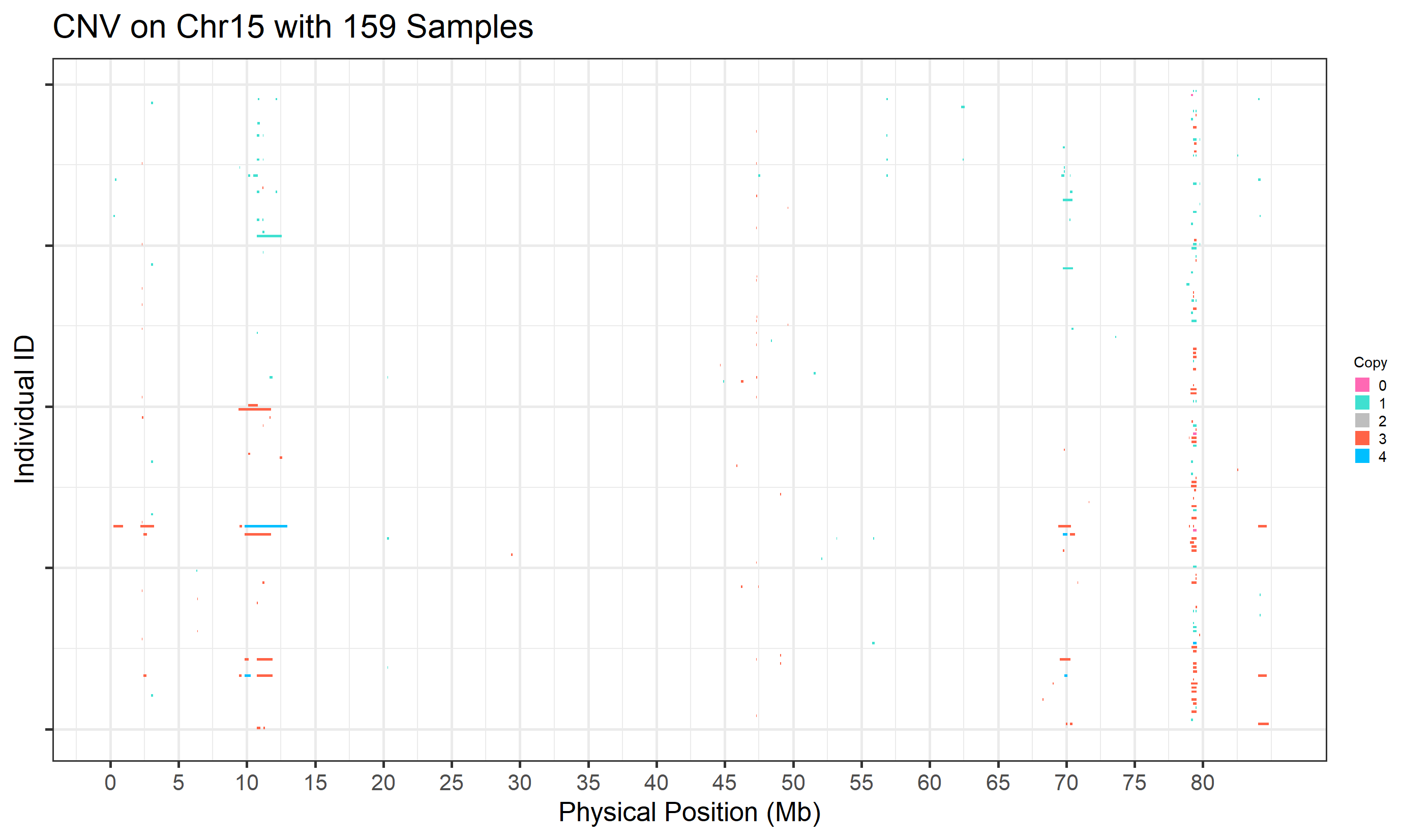
Figure.1 CNVs on Chromosome 15 (ARS reference) from PennCNV
Let’s now visualise CNVs from the CNVPartition results by chromosome. We can adjust the size of final figure by setting ‘width_1’ and ‘height_1’.
cnv_visual(clean_cnv = cnv_part_umd, #generated by 'cnv_clean' function in section 1
           max_chr = 29, #select how many Chromosomes to plot
           width_1 = 20, #optional,adjust the width of final plot
           height_1 = 12, #optional,adjust the height of final plot
           folder = "cnv_visual_all_part", )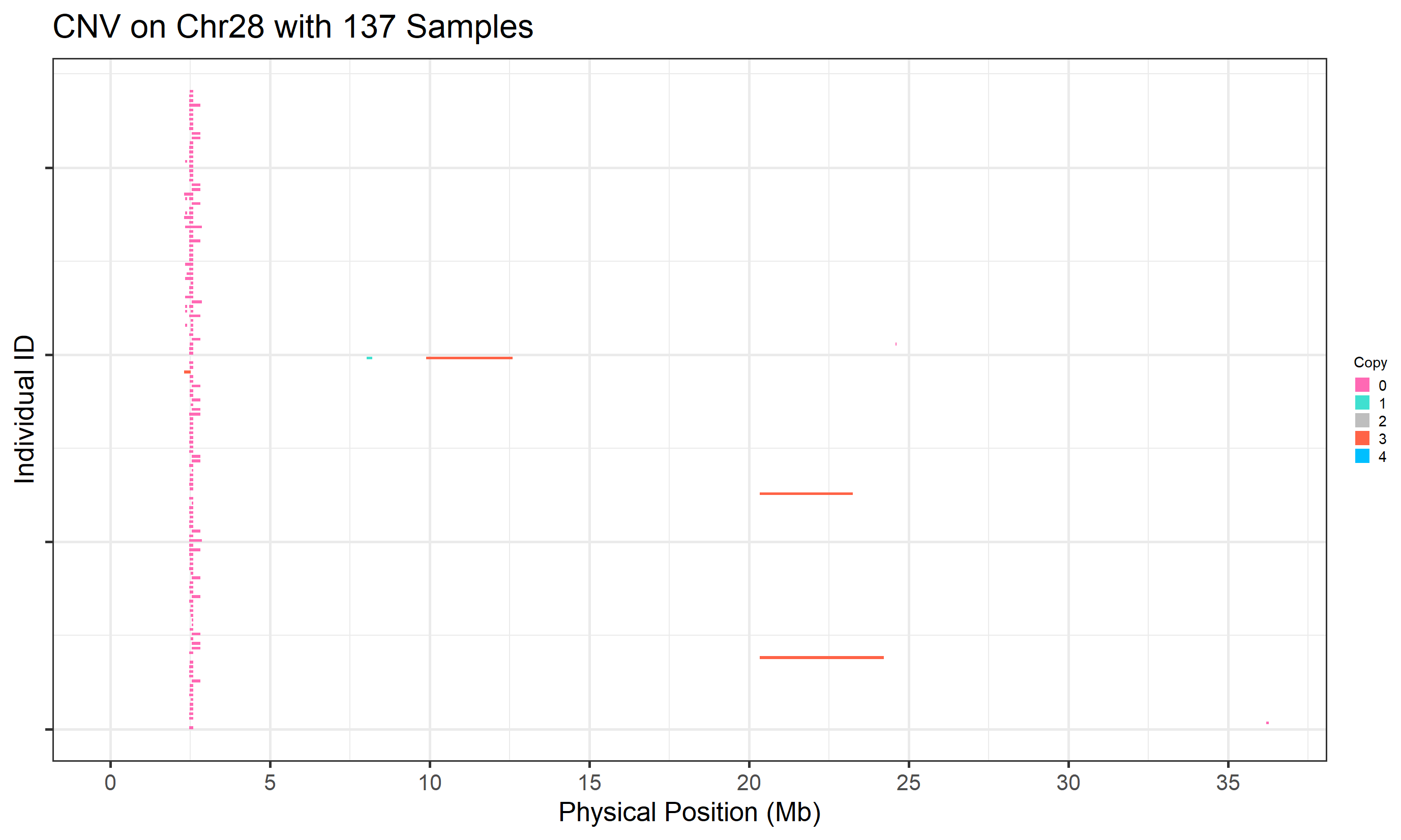
Figure.2 CNVs on Chromosome 28 (UMD reference) from CNVPartition
2.2 How do we plot CNVs in a region of interest?
After plotting all CNVs on each chromosome, we might find that some regions are particularly interesting. To plot these, we can add the options chr_id, start_position and end_position to the cnv_visual function call. Here, we are taking the region of Chr15:77-80.1221 Mb from the PennCNV results as an example.
cnv_visual(clean_cnv = cnv_penn_ars, #standard file was generated by 'cnv_clean' function in section 1
           chr_id = 15, #set Chromosome
           start_position = 77, #set start position, unit is 'Mb'
           end_position = 80.1221, #set end position, unit is 'Mb'
           col_0 = "red", #optional, customize colour for 0 copy CNVs
           col_1 = "orange", #optional, customize colour for 1 copy CNVs
           col_3 = "blue", #optional, customize colour for 3 copy CNVs
           col_4 = "green", #optional, customize colour for 4 copy CNVs
           width_1 = 13, #optional, adjust the width of final plot
           height_1 = 10, #optional, adjust the height of final plot
           folder = "cnv_visual")
#> Input data passed requirment check...
#> Task done, plot was stored in working directory.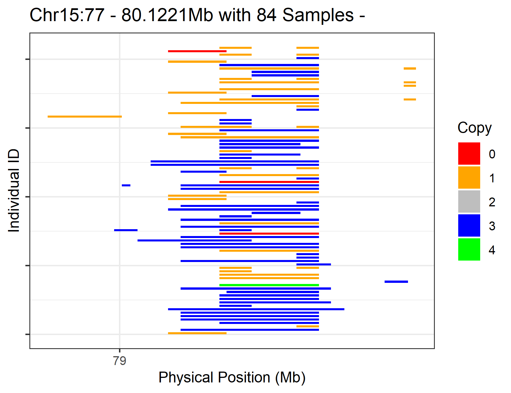
Figure.3 CNVs on Chr15:77-80.1221 Mb
2.3 How do we plot CNVs in a sample of interest?
Here we need to assign both the Sample ID (to individual_id) and the clean CNV list (to clean_cnv) in the cnv_visual function. The individual CNV plot will saved in the current working directory. For example, the sample “201094560076_R03C02” has the most CNVs in the PennCNV results, so let’s plot it and have a look. Note: we can use the individual_cnv_count.txt file (to be generated in section 3) to identify samples that exhibit large numbers of CNVs.
cnv_visual(clean_cnv = cnv_penn_ars, #standard file was generated by 'cnv_clean' function in section 1
           individual_id = "201094560076_R03C02", #set the sample ID
           width_1 = 20, #optional, adjust the width of final plot
           height_1 = 13, #optional. adjust the height of final plot
           folder = "cnv_visual")
#> Input data passed requirment check...
#> Task done, plot was stored in working directory.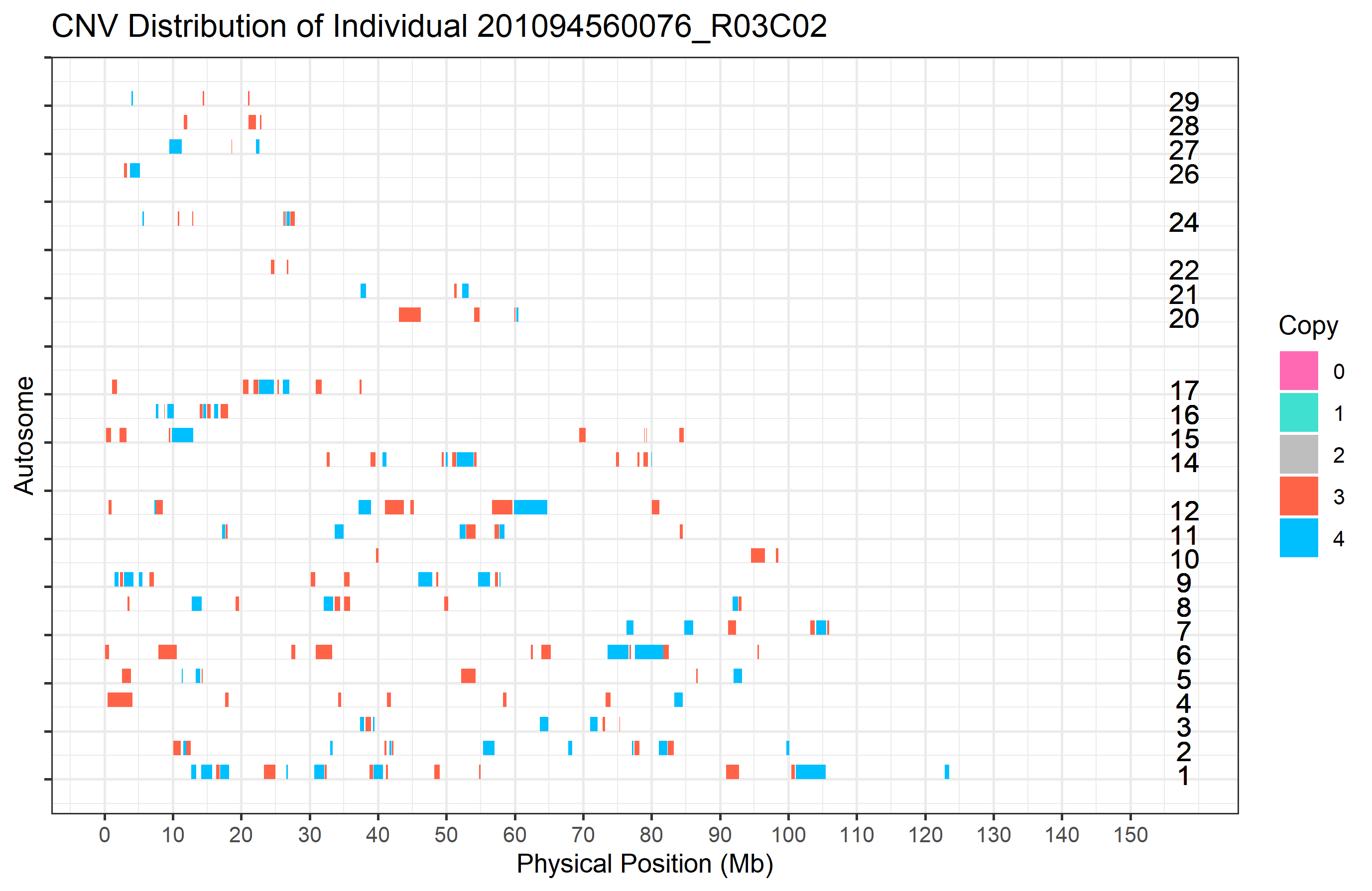
Figure.4 CNVs in a specific sample
2.4 How do we plot an interesting gene to see how many samples had a CNV overlapping with it?
The idea of plotting CNVs by target gene is to avoid making overly-strong statements when reporting important candidate genes after annotation for CNVRs. If we think that one particular gene is especially important in the CNV analysis, it’s better to present the frequency at which that gene has a structural variation in the experimental population. Plotting CNVs by gene will directly present how many samples show copy number variations overlapping the gene.
Note: The input file ‘cnv_annotation.txt’ will be generated in section 5.2, as part of annotating the gene to CNV results.
cnv_visual(clean_cnv = "call_gene_Penn_UCSC/cnv_annotation.txt", #here we need the annotated CNV list, generated by 'call_gene' in section 5.2
           target_gene = "BLA-DQB", #set the gene name we are interested in
           col_0 = "darkorchid4",  #optional, customize colour for o copy CNV
           col_1 = "dodgerblue3",  #optional, customize colour for 1 copy CNV
           col_3 = "violetred3",  #optional, customize colour for 3 copy CNV
           col_4 = "orangered3",  #optional, customize colour for 4 copy CNV
           width_1 = 13, #adjust the width of final plot
           height_1 = 10, #adjust the width of final plot
           folder = "cnv_visual")
#> Renamed 'CNV_Start' and 'CNV_End' as 'Start' and 'End', input data passed requirment check...
#> Task done, plot was stored in working directory.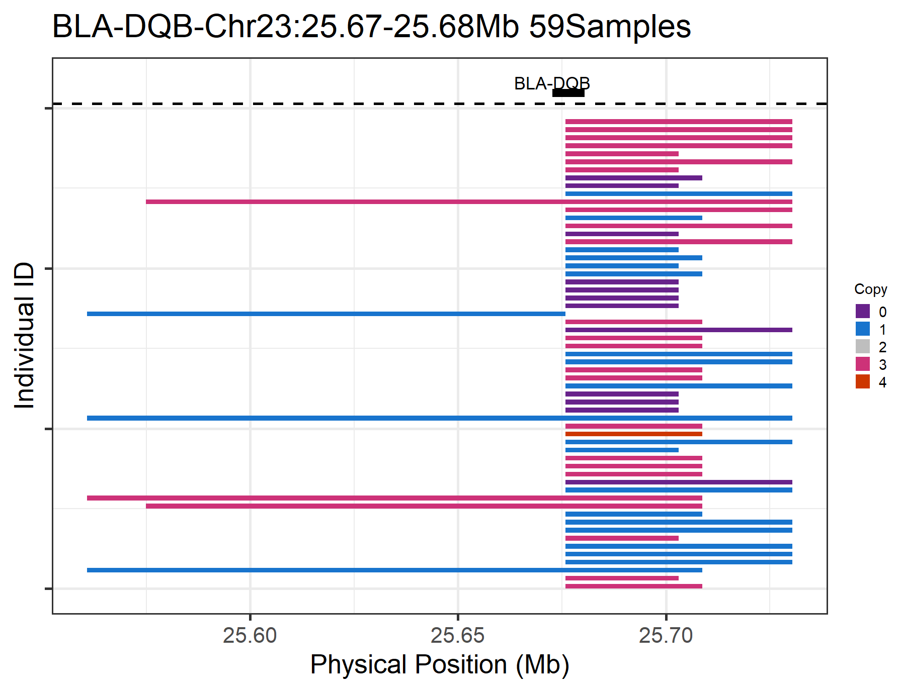
Figure.5 CNVs on a specific gene (BLA-DQB)
2.5 How can we present annotated genes above the CNV plot?
To do this, we need to provide two input files to the cnv_visual function: the CNV list in clean_cnv and gene annotations in refgene. We should also set the genomic region we are interested in. The reference gene list will be generated by the get_refgene function in section 5.
cnv_visual(clean_cnv = cnv_penn_ars, #standard file was generated by 'cnv_clean' function in section 1
           refgene = "refgene/Cow_ARS_UCSC.txt", #standard input file will generated by the function 'get_refgene' in Section 5
           chr_id = 23, #set Chromosome
           start_position = 25.56, #set start position, unit is 'Mb'
           end_position = 25.74, #set end position, unit is 'Mb'
           gene_font_size = 2.2, #optional, adjust the size of gene font
           show_name = c(25.66,27.72), #optional, show the gene in the given interval, maximum support two intervals
           col_0 = "tomato", #optional, customize colour for 0 copy CNV
           col_1 = "hotpink", #optional, customize colour for 1 copy CNV
           col_3 = "turquoise", #optional, customize colour for 3 copy CNV
           col_4 = "aquamarine", #optional, customize colour for 4 copy CNV
           col_gene = "red", #optional, customize colour of gene
           width_1 = 14, #optional, adjust the width of final plot
           height_1 = 10, #optional, adjust the height of final plot
           folder = "cnv_visual")
#> Input data passed requirment check...
#> [1] "CNV on Chromosome 23: 25.56 - 25.74 Mb with 68 Individual - "
#> Plotting gene...
#> Task done, plot was stored in working directory.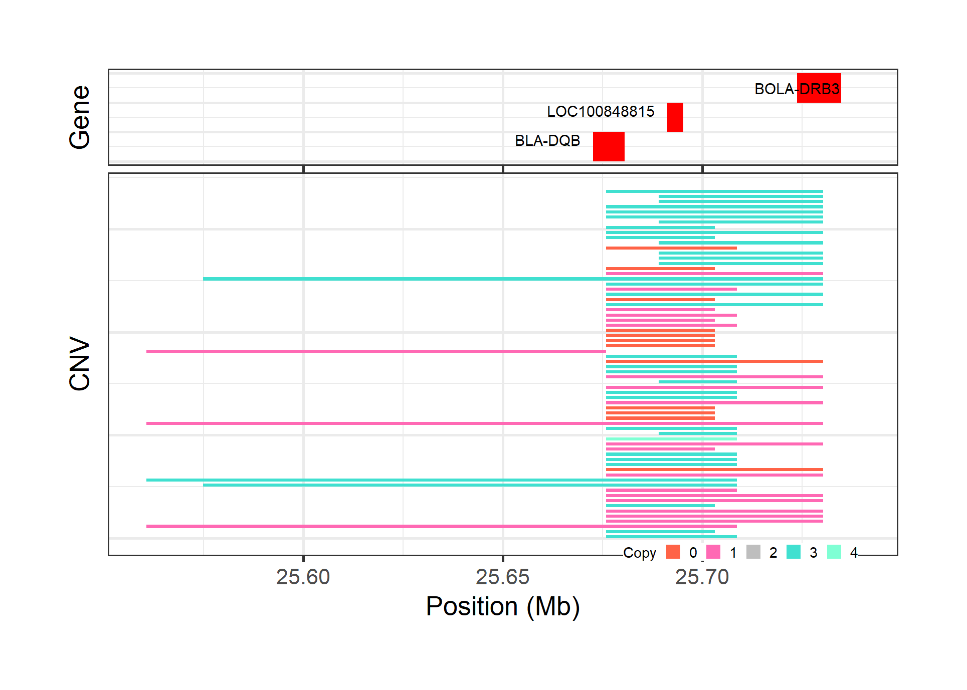
Figure.6 CNVs with annotated genes
3. What types of summary plots are available?
Using the clean CNV results, we can run the cnv_summary_plot function to generate a range of summary plots. These plots can aggregate CNV results by length group, CNV type, chromosome, and individual. It is also possible to make two different types of plots combining these figures.
cnv_summary_plot(clean_cnv = cnv_penn_ars, #standard file was generated by 'cnv_clean' function in section 1
                 length_group = c(0.05, 0.1, 0.2, 0.3, 0.4, 0.5, 0.6, 0.7, 1, 2, 5), # optional, set group of vectors to divide CNV length, unit is Mb. such as vector of ‘c(0.05, 0.3, 1)’, means divide the CNV length into four group: '<0.05Mb', '0.05 - 0.3Mb', '0.3-1Mb' and '>1Mb', maximum can accept 11 valueses
                 col_0 = "red", #optional, customize color for o copy CNV
                 col_1 = "black", #optional, customize color for o copy CNV
                 col_3 = "purple", #optional, customize color for o copy CNV
                 col_4 = "blue", #optional, customize color for o copy CNV
                 plot_sum_1 = TRUE,  #optional, make sum combination plot 1
                 height_sum1 = 26, #optional, adjust the size of sum plot 1
                 width_sum1 = 20, #optional, adjust the size of sum plot 1
                 plot_sum_2 = TRUE, #optional, make sum combination plot 2
                 height_sum2 = 20, #optional, adjust the size of sum plot 2
                 width_sum2 = 27, #optional, adjust the size of sum plot 2
                 folder = "cnv_summary_plot_penn")
#> Deviding the length group...
#> Plotting...
#> The CNV distribution plot has been saved in the 'cnv_summary_plot_penn' directory.
#> The CNV length group plot was saved in the 'cnv_summary_plot_penn' directory.
#> The box plot of CNV lengths was saved in the 'cnv_summary_plot_penn' directory.
#> Distribution of CNV type on chromosome plot was saved in working directory.
#> The number of CNV in Individual plot was saved in working directory.
#> cnv_summary_plot_1 was saved in working directory.
#> cnv_summaray_polt_2 was saved in working directory.
#> Task done.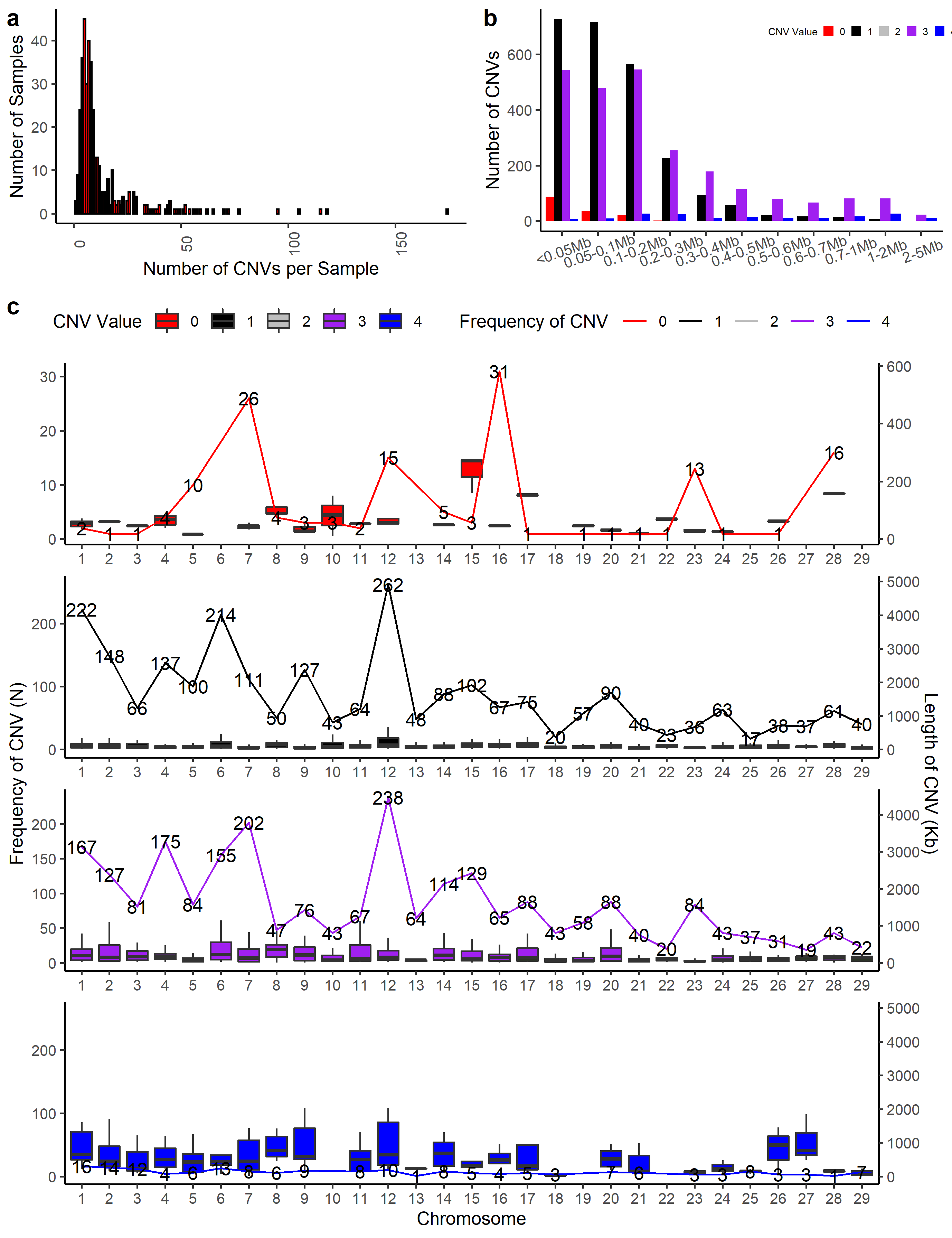
Figure.7 CNV Summary Plot Combination 1
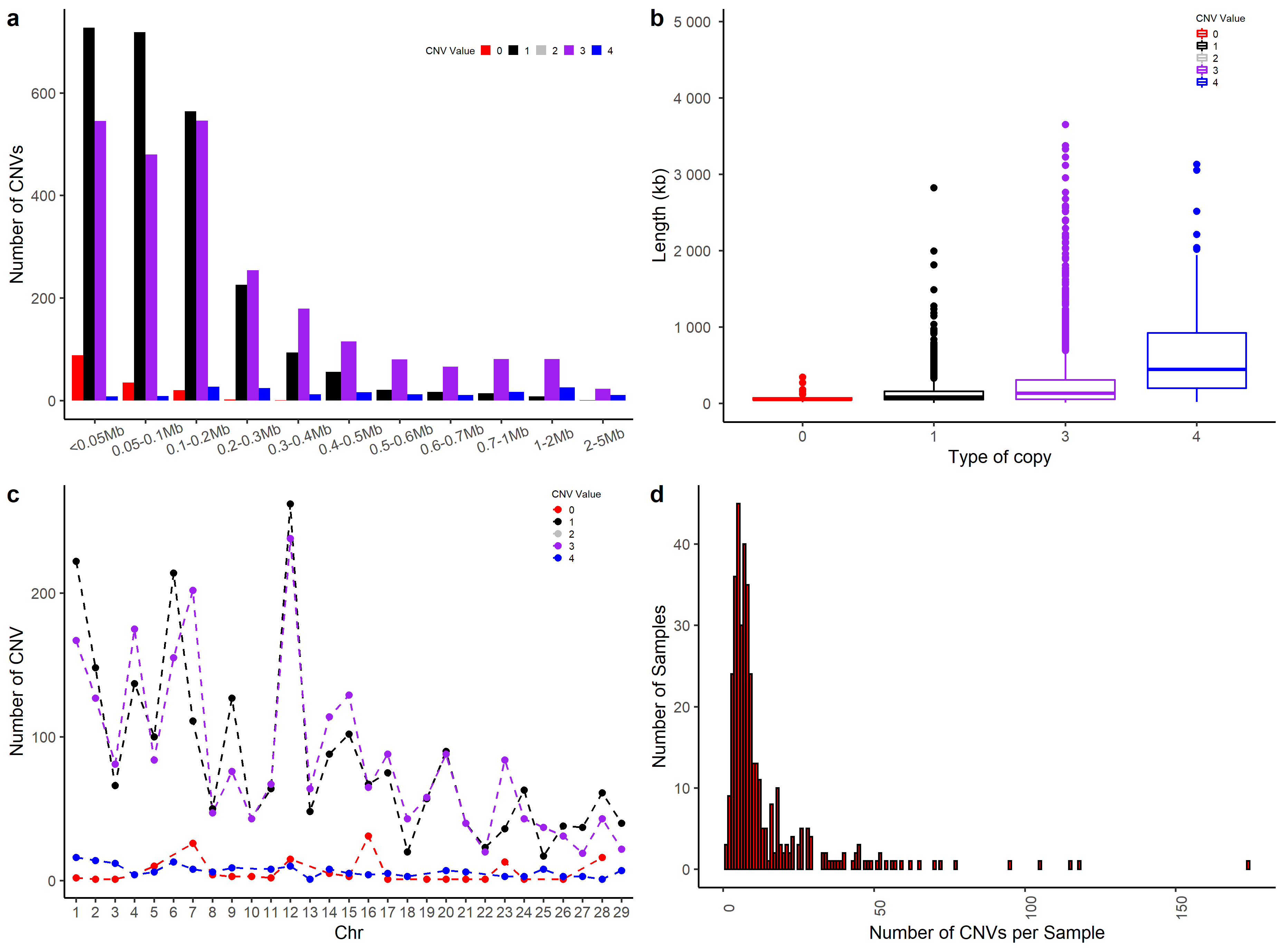
Figure.8 CNV Summary Plot Combination 2
4. How do we generate CNVRs (CNV Regions) from CNV results?
CNV regions are defined as regions of the genome containing one or more CNVs that overlap by at least one base pair: s a result, CNVRs will never overlap one another. As an example, let’s first generate CNVRs for the clean PennCNV results, using the call_cnvr function. A key parameter of this function is chr_set, which allows setting the maximum number of chromosomes over which to generate CNVRs. In our example, the species is Bos taurus (cows), with 29 autosomes, so we set chr_set = 29. This function will output three tables:
- The list of CNVRs. This is saved into the file
individual_cnv_cnvr.txt. - A brief summary table showing numbers of CNVRs by length and type (Deletion, Duplication, and Mixed). Mixed indicates that both duplications and deletions are found within the CNVR.
- The total length and number of CNVRs on each chromosome.
The resulting CNVRs are sorted by chromosome, start position, and end position, then assigned the CNVR ID to each unique interval by order. One of the output files, individual_cnv_cnvr.txt contain both CNVR and CNV information for every sample: this file might suitable for CNV-GWAS analyses.
cnvr_penn_ars <- call_cnvr(clean_cnv = cnv_penn_ars, #standard file was generated by 'cnv_clean' function in section 1
                  chr_set = 29, #Set the maximum number of chromosomes (29 autosomes for cattle)
                  folder = "call_cnvr_penn")
#> Chromosome 1 has been processed.
#> Chromosome 2 has been processed.
#> Chromosome 3 has been processed.
#> Chromosome 4 has been processed.
#> Chromosome 5 has been processed.
#> Chromosome 6 has been processed.
#> Chromosome 7 has been processed.
#> Chromosome 8 has been processed.
#> Chromosome 9 has been processed.
#> Chromosome 10 has been processed.
#> Chromosome 11 has been processed.
#> Chromosome 12 has been processed.
#> Chromosome 13 has been processed.
#> Chromosome 14 has been processed.
#> Chromosome 15 has been processed.
#> Chromosome 16 has been processed.
#> Chromosome 17 has been processed.
#> Chromosome 18 has been processed.
#> Chromosome 19 has been processed.
#> Chromosome 20 has been processed.
#> Chromosome 21 has been processed.
#> Chromosome 22 has been processed.
#> Chromosome 23 has been processed.
#> Chromosome 24 has been processed.
#> Chromosome 25 has been processed.
#> Chromosome 26 has been processed.
#> Chromosome 27 has been processed.
#> Chromosome 28 has been processed.
#> Chromosome 29 has been processed.
#> 978 CNVRs generated in total.
#> Overall summary of CNVRs:
#> # A tibble: 3 x 6
#>   Type      N `Average Length` `Min Length` `Max Length` `Total Length`
#>   <chr> <int>            <dbl>        <dbl>        <dbl>          <dbl>
#> 1 Gain    347           150153         7947      2639041       52103038
#> 2 Loss    399           100664         3703       737404       40164889
#> 3 Mixed   232           898204         6735      8282577      208383407
#> Summary of CNVRs on each Chromosome:
#> # A tibble: 29 x 3
#>    Chr   `Total Length` `Number of CNVR`
#>    <chr>          <dbl>            <int>
#>  1 1           26386484               62
#>  2 10           6784489               35
#>  3 11          12434667               33
#>  4 12          23045567               34
#>  5 13           4035800               35
#>  6 14          11313259               31
#>  7 15          10540774               32
#>  8 16           9051167               31
#>  9 17          12211360               32
#> 10 18           3455220               35
#> # ... with 19 more rows
Next, let’s generate CNVRs for CNVPartition and standard CNV lists. In order to avoid mixing the results among different files, we can set the folder argument to assign a distinguishing name to the newly generated folder.
5. How do we annotate genes for CNVRs and CNVs?
Once we have defined some CNV regions, we might want to see how many genes are located each. We can annotate genes to both CNVs and CNVRs using the call_gene function. Before that, however, we need to prepare gene lists for the correct reference genome. This can be done using the get_refgene function, as described in the following sections.
5.1 How do we download the reference gene lists we need?
We can use the get_refgene function to automatically download the reference gene list and convert it to the standard format required for functions such as call_gene. First, let’s run get_refgene without arguments to see which reference gene lists we can download. If you don’t find the information you’re looking for, please feel free to contact our maintainer to update it to you. For now, only reference gene lists from the UCSC website are supported; however, we may add more features if there is sufficient demand.
get_refgene()
#> Please select which version to download from following list:
#>  [1] "Cow_ARS_UCSC"            "Cow_ARS_ENS"
#>  [3] "Cow_UMD_UCSC"            "Pig_susScr11_UCSC"
#>  [5] "Pig_susScr11_ENS"        "Human_hg38"
#>  [7] "Human_hg19"              "Sheep_Oar_v4.0_UCSC"
#>  [9] "Sheep_Oar_v3.1_UCSC"     "Sheep_Oar_v3.1_ENS"
#> [11] "Horse_equCab3.0_UCSC"    "Horse_equCab2.0_UCSC"
#> [13] "Dog_UMICH_Zoey_3.1_UCSC" "Dog_UMICH_Zoey_3.1_ENS"
#> [15] "Chicken_galGal6_UCSC"    "Chicken_galGal5_UCSC"
Now, let’s get the reference gene list for the PennCNV results. This dataset was generated using ARS-UCD 1.2 as reference genome. Two gene lists are available for this reference: cow_ARS_UCSC and cow_ARS_ENS. The suffix ENS indicates the Ensembl reference gene list. The gene list will be saved in the folder refgene, which will be created first if necessary.
Cow_ARS_UCSC <- get_refgene(gene_version = "Cow_ARS_UCSC")
#> Link to the website...
#> Converting format...
#> Task done.
Cow_ARS_ENS <- get_refgene(gene_version = "Cow_ARS_ENS")
#> Link to the website...
#> Converting format...
#> Task done.
Next let’s get reference gene list for the CNVPartition and Standard result sets, both of which were generated on the UMD 3.1 reference genome; in this case, Cow_UMD_UCSC is the correct option to select.
COW_UMD_UCSC <- get_refgene(gene_version = "Cow_UMD_UCSC")
#> Link to the website...
#> Converting format...
#> Task done.
Now we have well-prepared reference gene lists, let’s return to the call_gene function.
5.2 The call_gene function
The call_gene function has three arguments:
-
ref_gene: this argument is required, and takes the path of a downloaded gene set (in therefgenefolder). -
interval: an optional file containing a list of CNV regions. This argument can also point to any file storing interval data in the correct format; examples could include CRVs, QTL windows, or haplotype lists. -
clean_cnv: an optional file containing a list of CNVs
We suggest that both ‘interval’ and ‘clean_cnv’ should be set simultaneously: this will enable reporting of the frequency of all annotated genes by counting how many CNVs overlapped to each gene within a CNVR. In section 10, we will show how to use the output file gene_freq_cnv.txt to make comparisons between different CNV results to find sets of consensus genes.
As an example, we will first call genes for the PennCNV results, ensuring that the gene list for the correct reference has been set (ARS 1.2). In this case, we are using the Ensembl-provided gene list.
call_gene(refgene = "refgene/Cow_ARS_ENS.txt", #standard file was generated by 'get_refgene' function in section 5.1
          interval = cnvr_penn_ars, #optional, standard file was generated by 'call_cnvr' function in section 4
          clean_cnv = cnv_penn_ars, #optional, standard file was generated by 'cnv_clean' function in section 1
          folder = "call_gene_Penn_Ens")
#> Warning in call_gene(refgene = "refgene/Cow_ARS_ENS.txt", interval = cnvr_penn_ars, : The following genes are duplicated in multiple CNVRs, and will only be annotated on the first CNVR_ID in the final gene frequency list report!
We can also use the UCSC gene list:
call_gene(refgene = "refgene/cow_ARS_UCSC.txt", #standard file was generated by 'get_refgene' function in section 5.1
          interval = "call_cnvr_Penn/cnvr.txt", #standard file was generated by 'call_cnvr' function in section 4
          clean_cnv = "cnv_clean/penncnv_clean.cnv", #optional, standard file was generated by 'cnv_clean' function in section 1
          folder = "call_gene_Penn_UCSC")
#> Warning in call_gene(refgene = "refgene/cow_ARS_UCSC.txt", interval = "call_cnvr_Penn/cnvr.txt", : The following genes are duplicated in multiple CNVRs, and will only be annotated on the first CNVR_ID in the final gene frequency list report!
Comparing the results, we observe that the results from two reference gene lists are slightly different, likely because the maintainers of each database have different methodologies (and possibly data sources) for producing their gene annotations. As a result of this, the position and quantity of genes might slightly differ between gene builds even for the same reference genome. Therefore, it may be important to validate genes of interest in more than one database.
Now, let’s call genes for the CNVPartition results. As before, we provide both CNVR and CNV lists, and set the new folder name by arguments. Note that we need to use the UMD 3.1 reference build for this data set. We also run the standard CNV set (using the ARS1.2 reference).
call_gene(refgene = "refgene/cow_UMD_UCSC.txt", #standard file was generated by 'get_refgene' function in section 5.1
          interval = "call_cnvr_Part/cnvr.txt", #standard file was generated by 'call_cnvr' function in section 4
          clean_cnv = "cnv_clean/cnvpart_clean.cnv", #optional, standard file was generated by 'cnv_clean' function in section 1
          folder = "call_gene_Part")
#> Warning in call_gene(refgene = "refgene/cow_UMD_UCSC.txt", interval = "call_cnvr_Part/cnvr.txt", : The following genes are duplicated in multiple CNVRs, and will only be annotated on the first CNVR_ID in the final gene frequency list report!
call_gene(refgene = "refgene/cow_ARS_UCSC.txt", #standard file was generated by 'get_refgene' function in section 5.1
          interval = "call_cnvr_standard/cnvr.txt", #standard file was generated by 'call_cnvr' function in section 4
          clean_cnv = "cnv_clean/cleancnv.cnv", #optional, standard file was generated by 'cnv_clean' function in section 1
          folder = "call_gene_standard_ARS_UCSC")
#> Warning in call_gene(refgene = "refgene/cow_ARS_UCSC.txt", interval = "call_cnvr_standard/cnvr.txt", : The following genes are duplicated in multiple CNVRs, and will only be annotated on the first CNVR_ID in the final gene frequency list report!
6. How to plot CNVR distribution map?
The function cnvr_plot is used to plot the CNVR distribution across chromosomes. For this function, we only need to assign the a CNVR list file to the cnvr argument, and the reference genome assembly to the assembly argument (to provide chromosome lengths). For Bovine data, we provide data for both ARS and UMD. For other species with data available (see the ref_gene function in section 5.1), we can just assign the species name to the assembly argument, for example, assembly = "hg38" for human data.
First, we’ll plot the CNVR distribution for the PennCNV data set. The default legend position might not suitable for all species; the arguments legend_x and legend_y can be used to move it if necessary.
cnvr_plot(cnvr = "call_cnvr_Penn/cnvr.txt", #standard file was generated by 'call_cnvr' function in section 4
          assembly = "ARS", #cattle could select 'UMD' or 'ARS', other species could assign the name of species
          loss_col = "green2", #optional, adjust the color of Loss type of CNVR
          gain_col = "red", #optional, adjust the color of Gain type of CNVR
          mixed_col = "black",  #optional, adjust the color of Mixed type of CNVR
          legend_x = 127, #optional, adjust the horizontal position of legend
          legend_y = 30,  #optional, adjust the vertical position of legend
          #height_1 = 14, #optional, adjust the height of CNVR plot
          #width_1 = 10, #optional, adjust the width of CNVR plot
          folder = "cnvr_plot_penn")
#> Task done, CNVR Distribution Plot saved in working directory.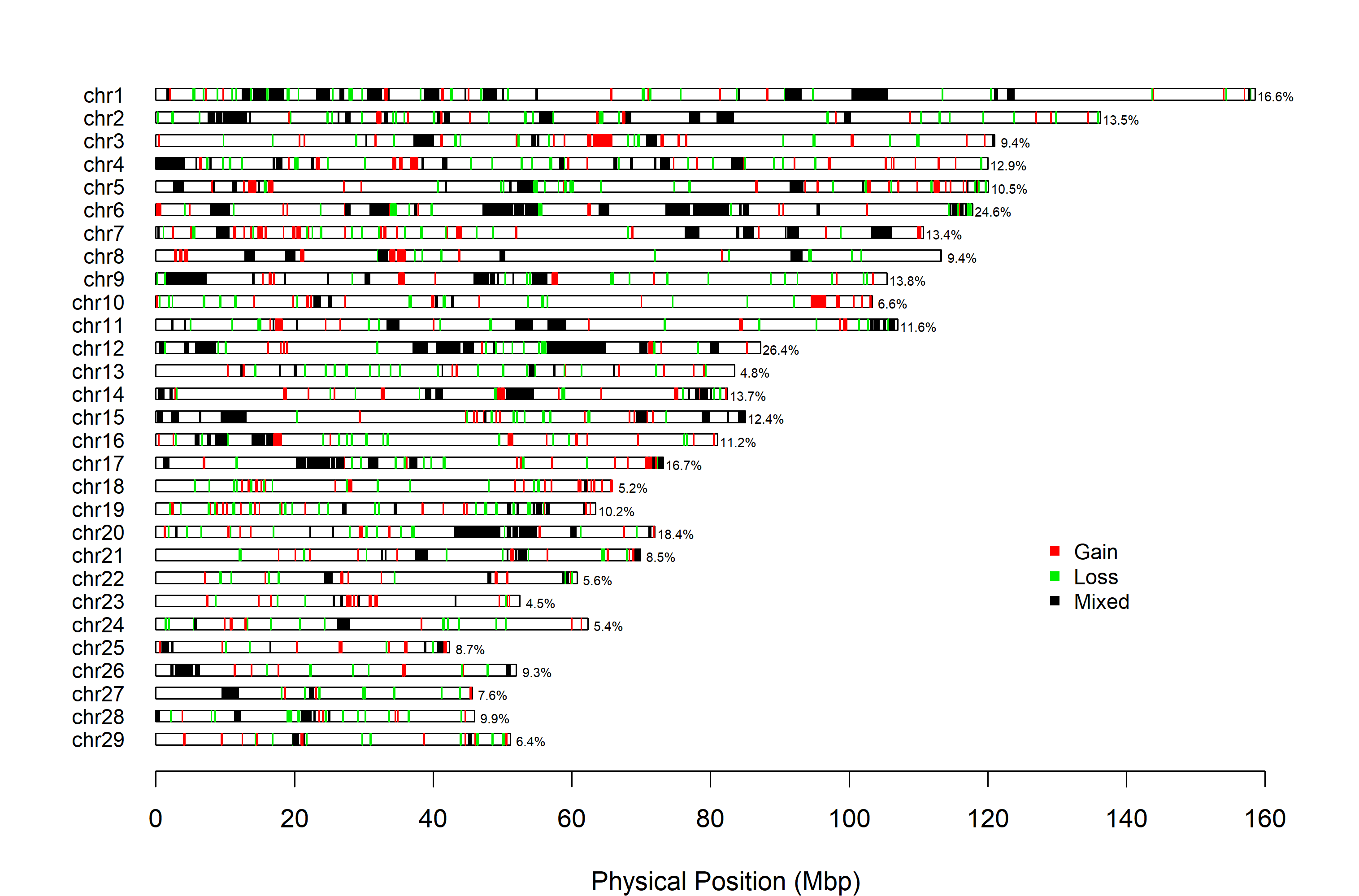
Figure.9 CNVR distribution map for PennCRV data
Next, we plot the CNVRs derived from the CNVPartition data set.
cnvr_plot(cnvr = "call_cnvr_Part/cnvr.txt", #standard file was generated by 'call_cnvr' function in section 4
          assembly = "UMD", #cattle could select 'UMD' or 'ARS', other species could assign the name of species
          loss_col = "darkorchid", #optional, adjust the color of Loss type of CNVR
          gain_col = "gold", #optional, adjust the color of Gain type of CNVR
          mixed_col = "tomato",  #optional, adjust the color of Mixed type of CNVR
          legend_x = 127, #optional, adjust the horizontal position of legend
          legend_y = 30,  #optional, adjust the vertical position of legend
          height_1 = 14, #optional, adjust the height of CNVR plot
          width_1 = 17, #optional, adjust the width of CNVR plot
          folder = "cnvr_plot_part")
#> Task done, CNVR Distribution Plot saved in working directory.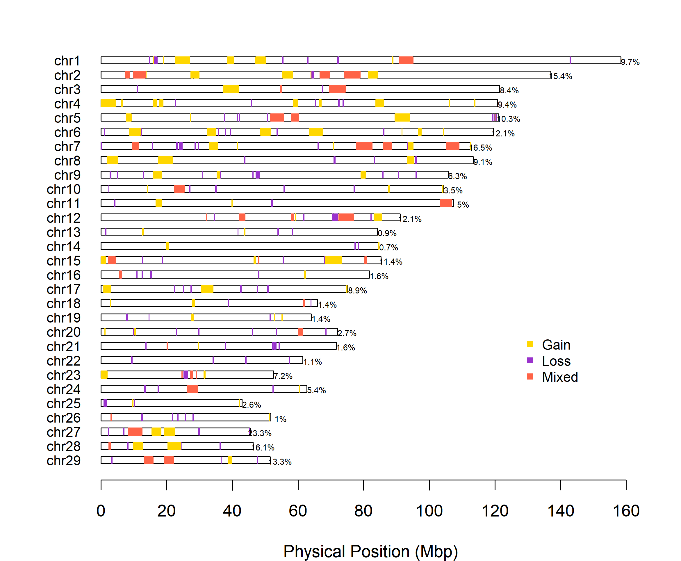
Figure.10 Part CNVR Distribution Map
7. How can we plot all high frequency CNVRs at once?
It always interesting to see which genomic regions have the highest frequencies of structure variation. To view these, we can plot all the high frequency regions using the cnvr_plot function.
As an example, let’s plot the PennCNV results. Remember to set a new folder name to save the results.
cnvr_plot(cnvr = "call_cnvr_Penn/cnvr.txt", #standard file was generated by 'call_cnvr' function in section 4
          clean_cnv = "cnv_clean/penncnv_clean.cnv", #standard file was generated by 'cnv_clean' function in section 1
          refgene = "refgene/cow_ARS_ENS.txt", #standard file was generated by 'get_refgene' function in section 5.1
          sample_size = 382, #total sample size
          common_cnv_threshold = 0.18, #the CNV frequency threshold
          width_1 = 10, #optional, adjust the width of final plot
          height_1 = 10, #optional, adjust the height of final plot
          col_gene = "blue", #optional, adjust the colour of annotated genes
          gene_font_size = 2.5, #optional, adjust the font size of annotated gene names
          folder = "high_freq_cnvr_penn")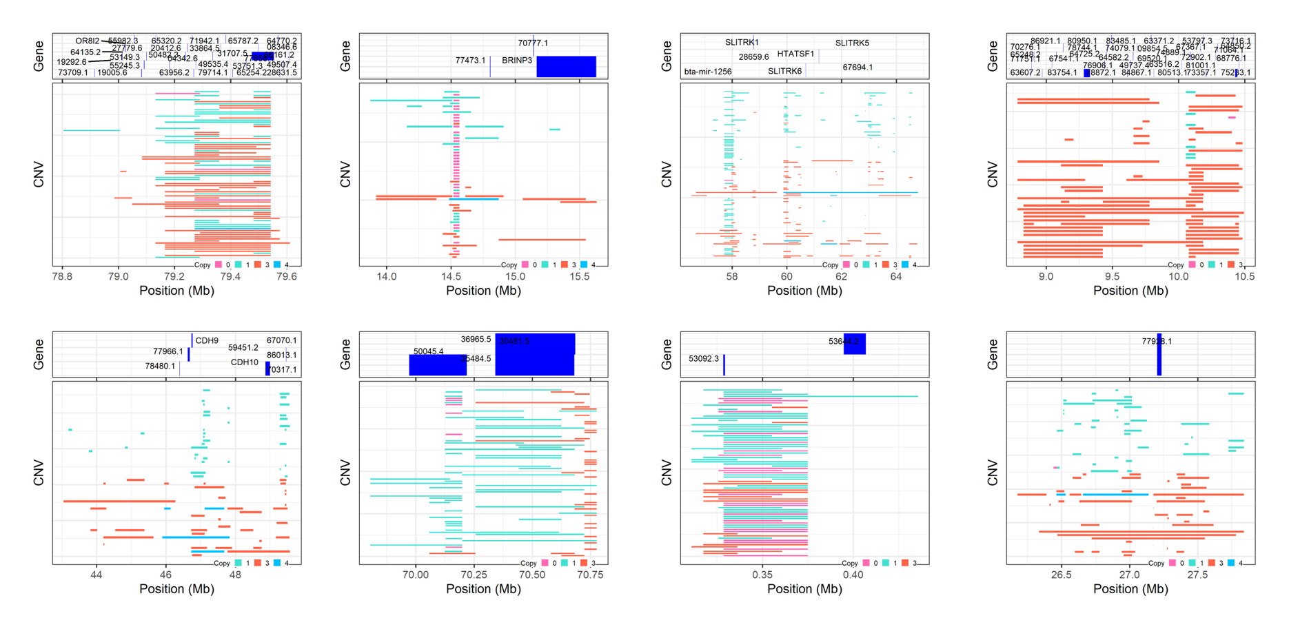
Figure.11 All high frequency CNVRs from PennCNV
8. Can we compare CNVs between different result sets?
Typically, we will use multiple models and software packages when predicting and analysing CNVs, especially when using data based on SNP chip genotypes. As a result, it is very common that we will need to compare two or more sets of predicted CNVs. To tackle this problem, we have implemented the compare_cnv function to make comparisons on both the individual and population levels. At the individual level, the function checks how many CNVs overlap in the same individual between two CNV result sets, thereby verifying the level of similarity between the two sets of results. On the population level, the comparison will check the level of overlap through the whole sample population, without checking whether or not the CNVs are present in the same individual; this can better indiciate the degree of repeatability of CNV detection between the two result sets.
As an example let’s compare the CNV prediction results for PennCNV and CNVPartition. Note that these results were generated using different reference builds, so the results of the comparison are currently rather meaningless (the physical coordinates of the CNVs will not line up across reference builds): this problem will be fixed in section 11 below.
compare_cnv(cnv_def = cnv_part_umd, #standard file was generated by 'cnv_clean' function in section 1
            cnv_tar = cnv_penn_ars, #standard file was generated by 'cnv_clean' function in section 1
            width_1 = 12, #optional, adjust the width of final plot
            height_1 = 11, #optional, adjust the height of final plot
            legend_x = 0.9, #optional, adjust the horizontal position of final plot
            legend_y = 0.9, #optional, adjust the vertical position of final plot
            col_1 = "pink", #optional, adjust the colour of Non-Overlapped part
            col_2 = "lightblue", #optional, adjust the colour of Overlapped part
            plot_caption = TRUE, #optional, show the Note information in plot or not
            folder = "compare_cnv_PartUMD_Vs_PennUMD")
#> [1] "Comparison Passed Validation, the number of Overlap and Non-overlap CNV equal to the original number of CNVs which are in total 1239"
#> [1] "The number of overlaped CNVs on individual level is 169, which is around 13.6 percent in the first file"
#> [1] "The number of Non-overlaped CNVs on individual level is 1070, which is around 86.4 percent in the first file"
#> [1] "Comparison to the first file was Passed Validation, the number of Overlap and Non-overlap CNV equal to the original number of CNVs which are in total of 1239"
#> [1] "The number of overlaped CNVs on population level is 541, which is around 43.7 percent in first file."
#> [1] "The number of Non-overlaped CNVs on population level is 698, which is around 56.3 percent in first file"
#> [1] "The final comparison results of the first file as follows: "
#>                  Item Individual.Level Population.Level
#> 1     Overlapped CNVs             13.6             43.7
#> 2 Non-overlapped CNVs             86.4             56.3
#> [1] "Comparison to the first file was finished."
#> [1] "Comparison to second file was Passed Validation, the number of Overlap and Non-overlap CNV equal to the original number of CNVs which are in total 5215"
#> [1] "The number of overlaped CNVs on individual level is 175, which is around 3.4 percent in second file."
#> [1] "The number of Non-overlaped CNVs on individual level is 5040, which is around 96.6 percent in second file."
#> [1] "Comparison to the second file was Passed Validation, the number of Overlap and Non-overlap CNV equal to the original number of CNVs which are in total of 5215"
#> [1] "The number of overlaped CNVs in seceond file on population level are 1379, which is around 26.4 percent"
#> [1] "The number of Non-overlaped CNVs in second file on population level are 3836, which is around 73.6 percent"
#> [1] "The final comparison results of the second file as follows: "
#>                  Item Individual.Level Population.Level
#> 1     Overlapped CNVs              3.4             26.4
#> 2 Non-overlapped CNVs             96.6             73.6
#> [1] "Task done. Comparison results were saved in your working directory"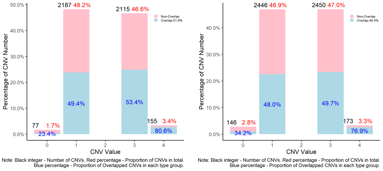
Figure.12 Comparison of PennCNV and CNVPartition results
9. What about CNVRs?
Similar to the compare_cnv function, we can use the compare_cnvr function to compare CNV regions. The same caveats apply with regard to the ensuring the two CNVR data sets were built on the same reference genome. Let’s try to use compare_cnvr now with the CNVPartition and Standard data sets (as before, ignoring for now the fact that these were produced on different reference genomes).
compare_cnvr(cnvr_def  = "call_cnvr_Part/cnvr.txt", #standard file was generated by 'call_cnvr' function in section 4
             cnvr_tar  = "call_cnvr_standard/cnvr.txt", #standard file was generated by 'call_cnvr' function in section 4
             width_1 = 8, #optional, adjust the width of comparison plot
             height_1 = 8, #optional, adjust the height of comparison plot
             hjust_prop = 0.2, #optional, adjust the horizontal position of the proportion number present in plot
             hjust_num = 1.6, #optional, adjust the horizontal position of the number present in plot
             col_1 = "grey15", #optional, adjust the colour of non-overlapped part
             col_2 = "forestgreen", #optional, adjust the colour of overlapped part
             folder = "compare_cnvr_PartUMD_Penn_UMD")
#> Comparison to the first file was Passed Validation, the number of Overlap and Non-overlap CNV equal to the original number of CNVRs which are in total of 246
#> CNVR comparison summary results in checkover_pop_1 as following:
#> # A tibble: 6 x 8
#> # Groups:   Type [3]
#>   Type  Check_overlap origi_length num_CNVR overlap_len num_overlap_oppsite
#>   <fct> <fct>                <int>    <int>       <dbl>               <int>
#> 1 Gain  Non-Overlap        1824550        7    53469808                   0
#> 2 Gain  Overlap          105638930       76    53993672                 100
#> 3 Loss  Non-Overlap        6194700       64     9566899                   0
#> 4 Loss  Overlap           11580677       64     8208478                  64
#> 5 Mixed Non-Overlap        3317779        4    36001939                   0
#> 6 Mixed Overlap           70606375       31    37922215                  60
#> # ... with 2 more variables: prop_overlap_len <dbl>, prop_num <dbl>
#> The number of overlaped CNVRs on population level is 171, which is around 69.5 percent in first file.
#> The number of Non-overlaped CNVRs on population level is 75, which is around 30.5 percent in first file
#> The overlapping length is 100124365 bp, which is around 50.3 percent in first file
#> The final comparison results of the first file as follows:
#>                   Item Number.of.CNVR Proportion.of.Number.... Length.bp.
#> 1     Overlapped CNVRs            171                     69.5  100124365
#> 2 Non-overlapped CNVRs             75                     30.5   99038646
#> 3             In Total            246                    100.0  199163011
#>   Proportion.of.Length....
#> 1                     50.3
#> 2                     49.7
#> 3                    100.0
#> Comparison to the first file was finished.
#> Comparison to the second file was Passed Validation, the number of Overlap and Non-overlap CNV equal to the original number of CNVRs which are in total of 878
#> CNVR comparison summary results in checkover_pop_2 as following:
#> # A tibble: 6 x 8
#> # Groups:   Type [3]
#>   Type  Check_overlap origi_length num_CNVR overlap_len num_overlap_oppsite
#>   <fct> <fct>                <int>    <int>       <dbl>               <int>
#> 1 Gain  Non-Overlap       35340763      238    36131115                   0
#> 2 Gain  Overlap           13315879       68    12525527                  68
#> 3 Loss  Non-Overlap       31958106      311    32810816                   0
#> 4 Loss  Overlap            6279030       51     5426320                  51
#> 5 Mixed Non-Overlap       70399922      107   117876424                   0
#> 6 Mixed Overlap          129649020      103    82172518                 106
#> # ... with 2 more variables: prop_overlap_len <dbl>, prop_num <dbl>
#> The number of overlaped CNVRs in seceond file on population level are 222, which is around 25.3 percent
#> The number of Non-overlaped CNVRs in second file on population level are 656, which is around 74.7 percent
#> The overlapping length is 100124365 bp, which is around 34.9 percent in second file
#> The final comparison results of the second file as follows:
#>                   Item Number.of.CNVR Proportion.of.Number.... Length.bp.
#> 1     Overlapped CNVRs            222                     25.3  100124365
#> 2 Non-overlapped CNVRs            656                     74.7  186818355
#> 3             In Total            878                    100.0  286942720
#>   Proportion.of.Length....
#> 1                     34.9
#> 2                     65.1
#> 3                    100.0
#> Processing the unique common CNVRs list by uniting overlepped CNVRs between two results
#> Chromosome 1 has been processed.
#> Chromosome 2 has been processed.
#> Chromosome 3 has been processed.
#> Chromosome 4 has been processed.
#> Chromosome 5 has been processed.
#> Chromosome 6 has been processed.
#> Chromosome 7 has been processed.
#> Chromosome 8 has been processed.
#> Chromosome 9 has been processed.
#> Chromosome 10 has been processed.
#> Chromosome 11 has been processed.
#> Chromosome 12 has been processed.
#> Chromosome 13 has been processed.
#> Chromosome 14 has been processed.
#> Chromosome 15 has been processed.
#> Chromosome 16 has been processed.
#> Chromosome 17 has been processed.
#> Chromosome 18 has been processed.
#> Chromosome 19 has been processed.
#> Chromosome 20 has been processed.
#> Chromosome 21 has been processed.
#> Chromosome 22 has been processed.
#> Chromosome 23 has been processed.
#> Chromosome 24 has been processed.
#> Chromosome 25 has been processed.
#> Chromosome 26 has been processed.
#> Chromosome 27 has been processed.
#> Chromosome 28 has been processed.
#> Chromosome 29 has been processed.
#> There are 168 unique and mutual CNVRs after uniting the overlapped CNVRs between two results
#> Task done. Comparison results were saved in the working directory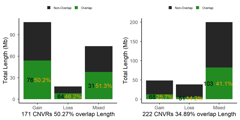
Figure.13 Comparison of CNVR
10. How do we find the consensus set of genes common to multiple CNV result sets?
One of the most interesting parts of CNV analysis is to find out which genes are affected by structure variations, and to check out the frequency of these aberrant genes in our samples. After using the call_gene function in section 5.2, we now have the gene frequency list for each CNV result set. We can take these lists as input in the compare_gene function to find the set of consensus genes common to multiple CNV results.
Now, let’s compare the annotated gene lists for the PennCNV and CNVPartition results as an example. We can assign the arguments gene_freq_1 and gene_freq_2 with the gene_freq_cnv.txt files from the call_gene_Part and call_gene_Penn output folders created earlier. Then we need to set an integer threshold (common_gene_threshold) for the number of observations required to declare that a gene is “commom”. In our example, the sample size is 400, so for a prevalence of 5%, the common_gene_threshold could calculated as 400 * 5% = 20.
compare_gene(gene_freq_1 = "call_gene_Part/gene_freq_cnv.txt", #standard file was generated by 'call_gene' function in Section 5.2
             gene_freq_2 = "call_gene_Penn_Ens/gene_freq_cnv.txt", #standard file was generated by 'call_gene' function in Section 5.2
             title_1 = "Bovine Part", #optional, adjust the title of input file 1 present in final plot
             title_2 = "Bovine Penn", #optional, adjust the title of input file 2 present in final plot
             common_gene_threshold = 20, #optional, the threshold is the gene frequency, here 20 means the Gene frequency exceed 20 in two input lists will be regarded as common gene.
             col_1 = "red", #optional, set the colour of 'Common High' genes
             col_2 = "blue", #optional, set the colour of 'Common Low' genes
             col_3 = "gold", #optional, set the colour of 'gene_freq_1'-only genes
             col_4 = "green", #optional, set the colour of 'gene_freq_2'-only genes
             height_1 = 10, #optional, adjust the height of final plot
             width_1 =  12, #optional, adjust the width of final
             folder = "compare_gene_Part_Vs_Penn")
#> [1] "Clustering common gene between the two input files..."
#> [1] "Brief summary of comparison as below:"
#> # A tibble: 4 x 2
#> # Groups:   Common_Gene [4]
#>   Common_Gene          n
#>   <chr>            <int>
#> 1 Common_High          5
#> 2 Common_Low        3029
#> 3 High_Freq_list_1     6
#> 4 High_Freq_list_2    54
#> [1] "Gene comparison list, brife summary and comparison plot was saved in working directory."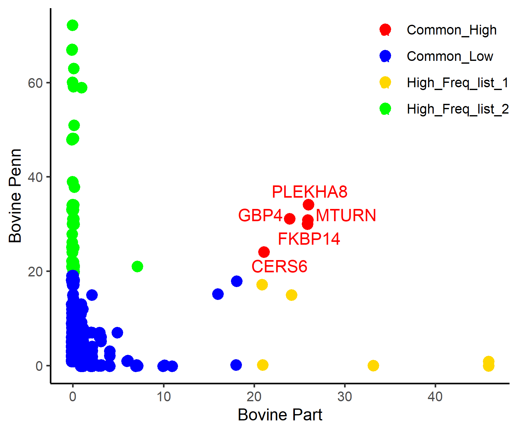
Figure.14 Comparison of genes present in the PennCNV (green) and CNVPartition (gold) gene lists
We can also compare the frequency lists for three genes, just by adding one more input file (using the gene_freq_3 argument); in this case, the comparison figure will be a 3D plot.
compare_gene(gene_freq_1 = "call_gene_Part/gene_freq_cnv.txt", #standard file was generated by 'call_gene' function in Section 5.2
             gene_freq_2 = "call_gene_Penn_Ens/gene_freq_cnv.txt", #standard file was generated by 'call_gene' function in Section 5.2
             gene_freq_3 = "call_gene_standard_ARS_UCSC/gene_freq_cnv.txt", #standard file was generated by 'call_gene' function in Section 5.2
             title_1 = "Part", #optional, adjust the title of input file 1 present in final plot
             title_2 = "ENS", #optional, adjust the title of input file 2 present in final plot
             title_3 = "UCSC", #optional, adjust the title of input file 3 present in final plot
             common_gene_threshold = 15,
             height_1 = 5.8, #optional, adjust the height of final plot
             width_1 = 5.8, #optional, adjust the width of final plot
             folder = "compare_gene_three_lists")
#> [1] "Starting merging gene lists..."
#> [1] "Clustering common gene among three gene lists..."
#> [1] "2 genes with higher frequency in all three gene lists, they are: "
#>    name2_1 Frequency_1 Frequency_2 Frequency_3 Common_Gene
#> 1:   CERS6          21          24          23 Common_High
#> 2:   STK39          21          17          19 Common_High
#> [1] "Brief summary:"
#> # A tibble: 3 x 2
#> # Groups:   Common_Gene [3]
#>   Common_Gene  Number_Gene
#>   <chr>              <int>
#> 1 Common_High            2
#> 2 Common_Low          3783
#> 3 High_and_Low         115
#> [1] "Gene comparison list, brife summary and comparison plot was saved in working directory."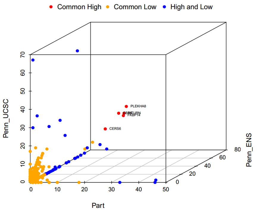
Figure.15 Comparison of three gene lists
If we add a fourth gene frequency lists, by adding the gene_freq_4 argument, the comparison figure produced will be a heat-map rather than a scatterplot.
compare_gene(gene_freq_1 = "call_gene_Part/gene_freq_cnv.txt", #standard file was generated by 'call_gene' function in Section 5.2
             gene_freq_2 = "call_gene_Penn_UCSC/gene_freq_cnv.txt", #standard file was generated by 'call_gene' function in Section 5.2
             gene_freq_3 = "call_gene_Part/gene_freq_cnv.txt", #standard file was generated by 'call_gene' function in Section 5.2
             gene_freq_4 = "call_gene_standard_ARS_UCSC/gene_freq_cnv.txt", #standard file was generated by 'call_gene' function in Section 5.2
             title_1 = "Part", #optional, adjust the title of input file 1 present in final plot
             title_2 = "ENS", #optional, adjust the title of input file 2 present in final plot
             title_3 = "UCSC", #optional, adjust the title of input file 3 present in final plot
             title_4 = "PUCSC", #optional, adjust the title of input file 4 present in final plot
             col_1 = "red", #optional, set the color of High frequency genes
             col_2 = "yellow", #optional, set the color of Low frequency genes
             common_gene_threshold = 20,
             height_1 = 9, #optional, adjust the height of final plot
             width_1 = 11, #optional, adjust the width of final plot
             folder = "compare_gene_four_lists")
#> Starting merging gene lists...
#> Clustering common gene among four gene lists...
#> 1 genes with higher frequency in all gene lists, they are:
#>    name2_1 Frequency_1 Frequency_2 Frequency_3 Frequency_4 Common_check
#> 1:   CERS6          21          24          21          23  Common_high
#> Brief summary:
#> # A tibble: 3 x 2
#> # Groups:   Common_check [3]
#>   Common_check Number_Gene
#>   <chr>              <int>
#> 1 Common_high            1
#> 2 Common_low          2401
#> 3 High_and_Low          34
#>
#> Gene comparison list, brife summary and comparison plot was saved in working directory.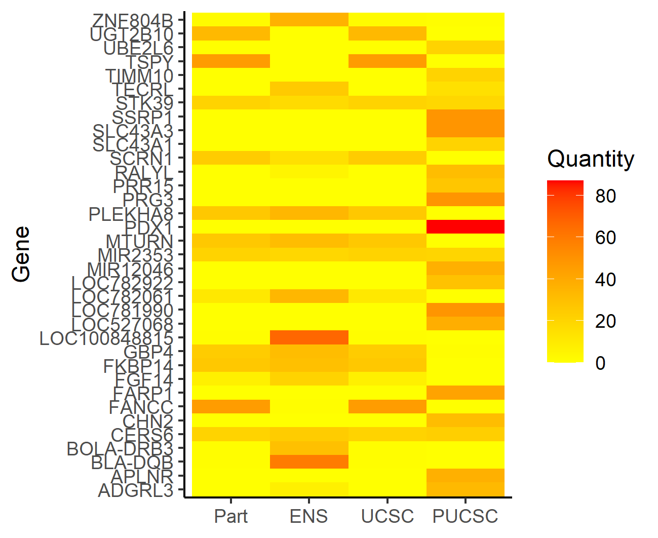
Figure.16 Heatmap comparing gene lists across four data sets
Brief summary
The ten functions we’ve run so far only require users to provide the CNV results, which can already generate plenty of summary results that include sufficient information to point us in the right direction to dig deeper. If we want to explore a particular region in more depth, there are extra functions in the HandyCNV package that can combine CNV data with other data sources. We will introduce some of these functions in the following section.
11. How can we create the map file used in HandyCNV, to allow comparing CNVs between different reference genomes?
We can use the convert_map function to prepare a map file; generally, we will need one for each reference file. In our examples, we have used the two bovine reference genomes ARS-UCD 1.2 and UMD 3.1. For HandyCNV, map files hould have the format shown in the table below, with the four columns Chromosome, SNP, MorganPos, and PhysicalPos. If the centiMorgan position (MorganPos) is unknown, we can assign the missing value as 0, or provide the phyisical position in megabases. This format is the same as the standard .map format used in Plink and other software, and can be exported from GenomeStudio. The column names are not required.
tabl <- "
-----------------------------------------
Chr   SNP           MorganPos PhysicalPos
---- ------------- ---------- -----------
  5   14636         56.3275   56327514
  5   16084         56.329    56328962
  5   19597         56.3325   56332475
  1   1_115292065   114.371   114370731
  1   1_115292107   114.371   114370773
-----------------------------------------"
Here, we have the map files for both bovine references included in the package, at the following paths:
ars_map <- system.file("extdata", "Demo_data/map/ARS1.2_GGPHDV3.map", package = "HandyCNV")
umd_map <- system.file("extdata", "Demo_data/map/UMD3.1_Bovine.map", package = "HandyCNV")
The function will not only generate map files, for use in compare_cnv and compare_cnvr, it will also generate map file used in Plink and PennCNV for both inputs. The conversion process also compares the two input maps and produces summary tables and figures.
convert_map(default_map = umd_map, #when running your own data, set this argument to 'default_map = "localpath/file"'
            target_map = ars_map, #when running your own data, set this argument to 'target_map = "localpath/file"'
            chr_set = 30,
            defMap_title = "UMD 3.1", #set the label of axis
            tarMap_title = "ARS-UCD 1.2", #set the label of axis
            col_1 = "green4", #set colour for the type of Match in SNP comparison plot
            col_2 = "red", #set colour for the type of Unmatched in SNP comparison plot
            col_3 = "deeppink2", #set colour for the bar of Target_Map in SNP density plot
            col_4 = "deeppink2", #set colour for line of Target_map in density plot
            col_5 = "turquoise3", #set colour for point of Default_Map in SNP density plot
            col_6 = "turquoise3", #set colour for line of Default_map in SNP density plot
            species = "Bovine",
            height_c = 16,
            width_c = 22,
            height_d = 14,
            width_d = 25)
#> [1] "Starting comparing the differences between the two versions"
#> [1] "Checking if negtive position exsits in new converted map...."
#>
#>  FALSE   TRUE
#> 139512    465
#> [1] "There are 465 SNPs with negtive postion in new assembly."
#> [1] "The matching results of SNP chromosome ID in the two versions are as follows:"
#>
#>    Match Mismatch
#>   122772    17211
#> [1] "The details of comparison as follows: "
#>                           Type.Var1 Type.Freq
#> 1           Both unknown Chromosome       344
#> 2              Different Chromosome       851
#> 3                   Same Chromosome    122428
#> 4            Unfound in Default map      2038
#> 5             Unfound in Target map         6
#> 6 Unknown Chromosome in Default map     13771
#> 7  Unknown Chromosome in Target map       545
#> [1] "Ploting SNP comparison results....."
#> [1] "Comparison of SNP by Chromosome plot was saved in working directory."
#> [1] "Preparing the map files for PennCNV and Plink...."
#> [1] "Writing converted map for PennCNV and Plink formats..."
#> [1] "Target map was converted to PennCNV map file..."
#> [1] "Converted map for PennCNV format were saved in working directory."
#> [1] "Converted map for Plink format were saved in working directory."
#> [1] "Plotting the Difference of SNPs between two versions of map..."
#> [1] "SNP difference plot was saved in working directory."
#> png
#>   2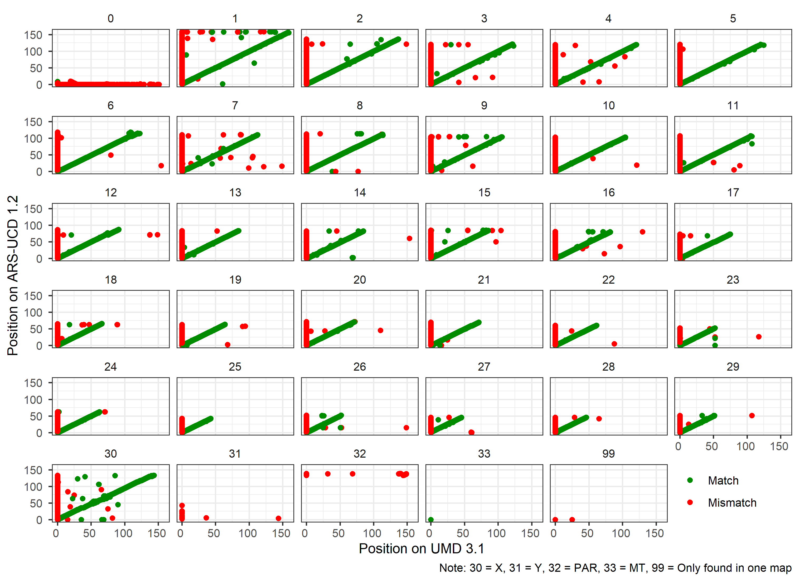
Figure.17 Comparison of the ARS 1.2 and UMD 3.1 reference genomes
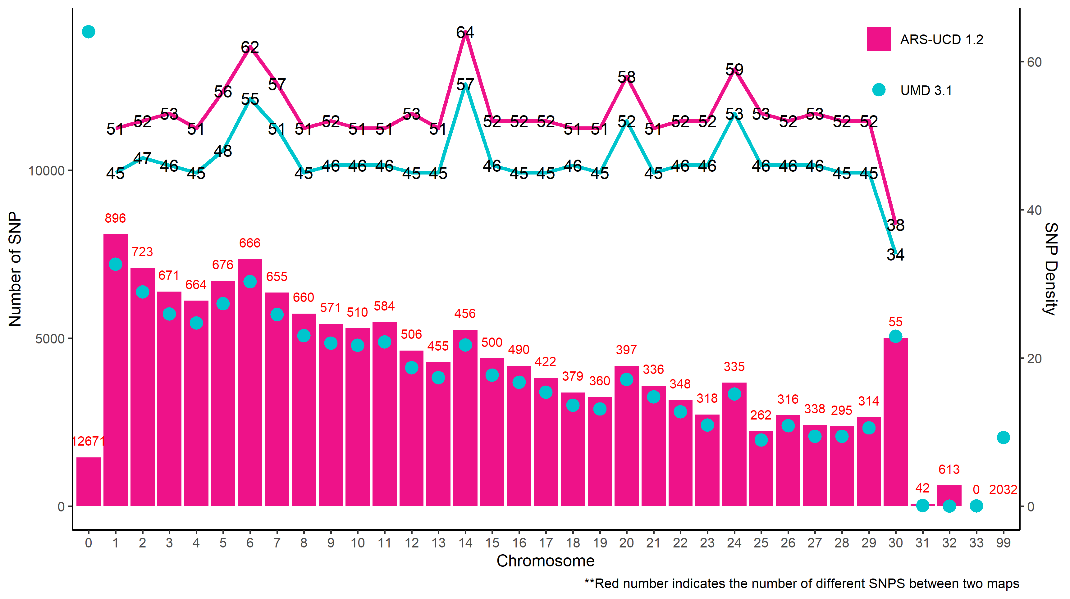
Figure.18 Comparison of SNP densities on the ARS 1.2 and UMD 3.1 maps
12. How can we integrate the CNVs and annotated genes with additional information, such as Log R ratio, B Allele Frequency, call rate, heterozygosity, missing value rate and Linkage Disequilibrium, and plot it as one figure?
The plot_cnvr_panorama function was built to achieve this task. But we need provide more information to this function: a. CNVR results(generated by ‘call_cnvr’ in section 4) b. Annotated CNV file (generated by ‘call_gene’ function) c. Signal Intensity file (In general it export from GenomeStudio which used in CNV detection process) d. Map file (Four columns used in Plink or generated by ‘convert_map’ function) e. Genotype files (generated by Plink with ‘–make-bed’ flag which include BED, BIM, FAM three files)
plot_cnvr_panorama(cnvr = "call_cnvr_Penn/cnvr.txt", #standard file was generated by 'call_cnvr' function in section 4
                   cnv_annotation = "call_gene_Penn_UCSC/cnv_annotation.txt", #standard file was generated by 'call_gene' function in Section 5.2
                   intensity = "Demo_data/demo_intensity.txt",
                   map = "Demo_data/demo.map",
                   prefix_bed = "Demo_data/demo_HandyCNV",
                   ld_heat = TRUE,
                   sample_size = 382,
                   common_cnv_threshold = 0.18,
                   col_0 = "green", #optional, customize color for o copy CNV
                   col_1 = "hotpink", #optional, customize color for 1 copy CNV
                   col_2 = "NA", #optional, customize color for 2 copy CNV
                   col_3 = "turquoise", #optional, customize color for 3 copy CNV
                   col_4 = "aquamarine", #optional, customize color for 4 copy CNV
                   col_gene = "red", #optional, customize color of gene
                   width_1 = 16,
                   height_1 = 30,
                   folder = "cnvr_panorama_heat_ld")
#> [1] "4 CNVRs passed the common frequency threshold."
#> Reading Demo_data/demo_HandyCNV.fam
#> Reading Demo_data/demo_HandyCNV.bim
#> Reading Demo_data/demo_HandyCNV.bed
#> ped stats and snps stats have been set.
#> 'p' has been set.
#> 'mu' and 'sigma' have been set.
#> [1] "Starting to make plot..."
#> [1] "Plot 1 (7_310937_435584_Mixed.png) was stored in the cnvr_panorama_heat_ld/ directory."
#> [1] "Plot 2 (15_78804694_79611716_Mixed.png) was stored in the cnvr_panorama_heat_ld/ directory."
#> [1] "Plot 3 (12_69804346_70777223_Mixed.png) was stored in the cnvr_panorama_heat_ld/ directory."
#> [1] "Plot 4 (12_56513728_64796304_Mixed.png) was stored in the cnvr_panorama_heat_ld/ directory."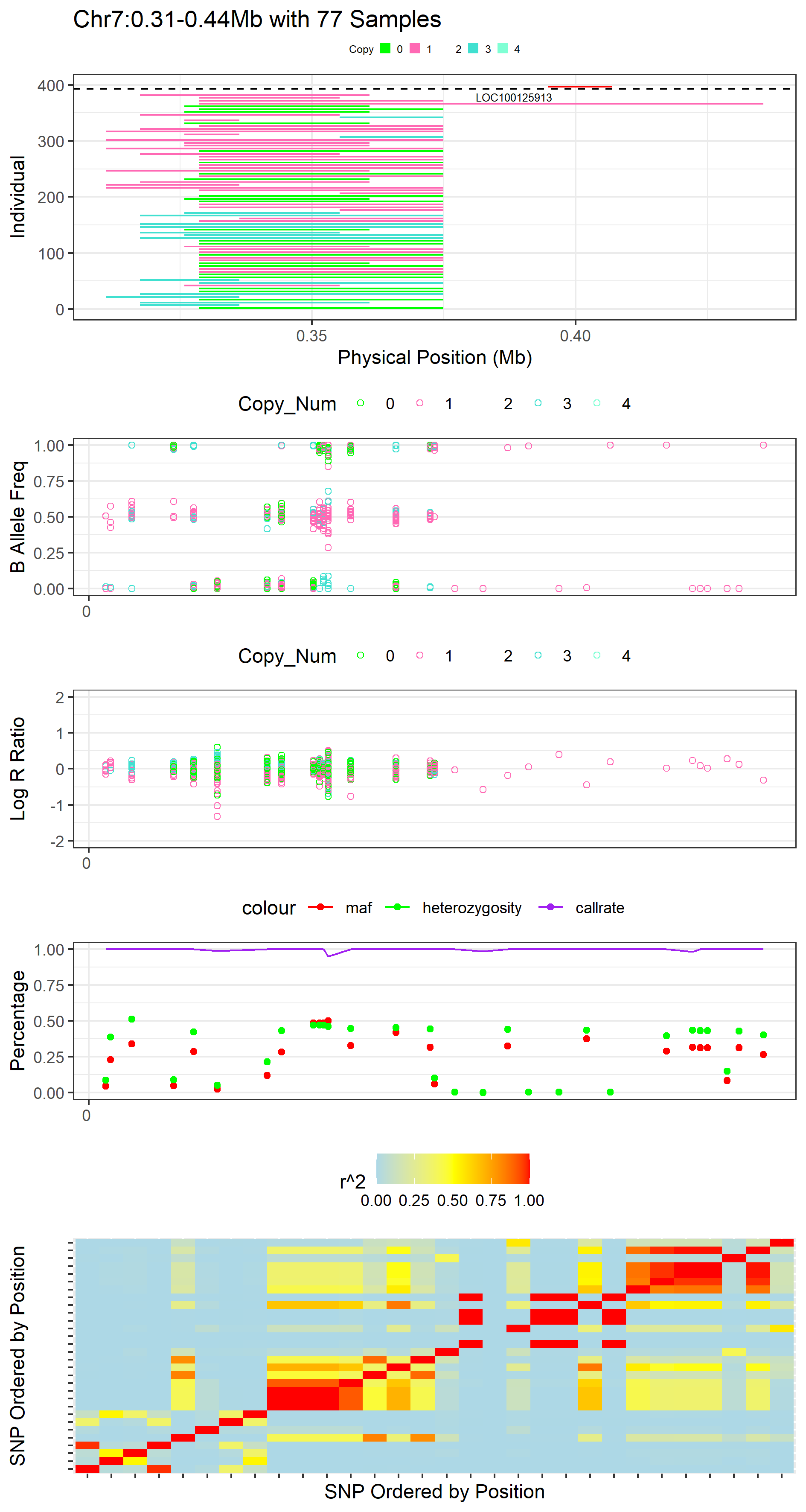
Figure.19 Example of CNVR Panorama with LD_Heatmap
For LD, we can replace the heatmap with the classic inverted triangle diagram by setting the argument ld_heat = FALSE, which will use the gaston package to plot LD. Because this requires converting the figure to ggplot format (via the ggplotify package), this process can be time consuming, and sometimes does not work well for large genomic regions. Therefore, we suggest that you use ld_heat = TRUE initially, before narrowing in on a particular region of interest to display with the classic LD plot.
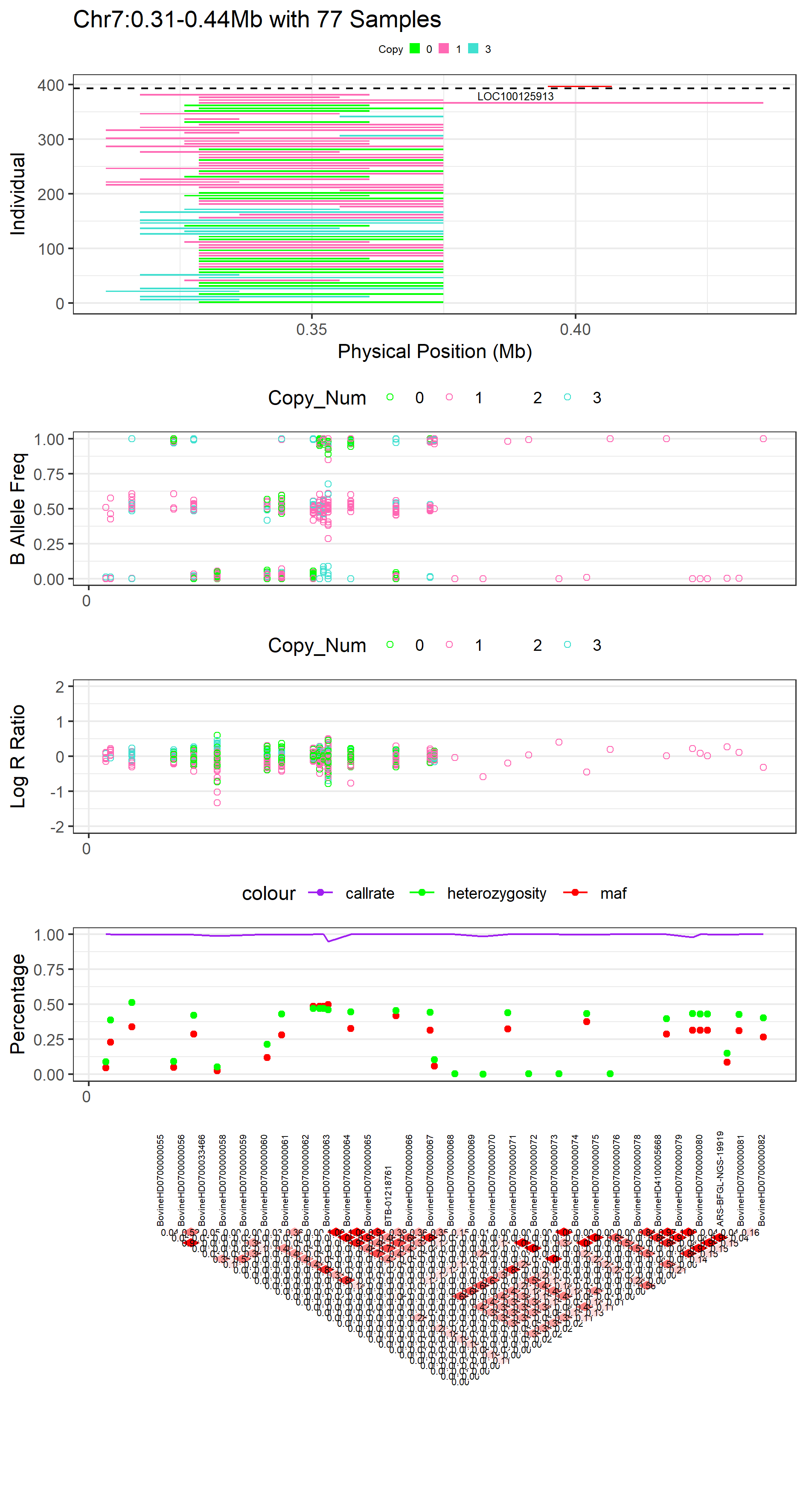
Figure.20 Example of CNVR Panorama with Classical_LD
13. How can we make a plot to show the source of the CNVs?
CNVs are heritable: with the pedigree information, particularly for the sires in a livestock context, we can produce plots of CNV sources. The plot_cnvr_source function can produce plots by sire, herd, and sire source. Sire source can be any freeform text, for example the country of origin. The expected input format is comma-separated (with a header), containing the following columns (in any order):
-
Chip_ID(matched to theSample_IDcolumn in the CNVR data) HerdSire_IDSire_Source
plot_cnvr_source(cnvr = "call_cnvr_Penn/cnvr.txt", #standard file was generated by 'call_cnvr' function in section 4
                clean_cnv = "cnv_clean/penncnv_clean.cnv", #standard file was generated by 'cnv_clean' function in section 1
                pedigree = system.file("extdata", "Demo_data/Pedigree/Pedigree.csv", package = "HandyCNV"),
                Frequent_threshold = 80,
                col_0 = "violet", col_1 = "turquoise", col_3 = "tomato", col_4 = "lightblue",
                report_id = T,
                height_1 = 20,
                width_1 = 15)
Figure.21 Plot Source of CNVR
14. How can we plot just the genes in a specific region, to save as a seperate figure?
The plot_gene function can do this for a specific reference gene set and genomic region.
plot_gene(refgene = "refgene/cow_ARS_UCSC.txt",
          chr_id = 7,
          start = 11,
          end = 12,
          height_1 = 3,
          width_1 = 10,
          show_name = c(11.0, 11.35, 11.75, 12.00),
          gene_font_size = 2.5)
#> png
#>   2
Figure.22 Gene plot
15. How can we find regions with high frequencies of runs of homozygosity?
An ROH (Run of homozygosity) is a region of an individual’s genome where almost all variants have homozygous genotypes. These regions generally indicate the presence of inbreeding in that individual’s ancestry, with more recent inbreeding leading to longer ROHs.
The function roh_window will produce two summary tables, as well as plotting the high frequency regions by chromosome. The first table summarises the total numbers and lengths of ROHs for each individual; the second reports summary statistics for aggregated windows of ROHs across all individuals.
roh_window(roh = "cnv_clean/cnvpart_roh.cnv",
           window_size = 2,
           length_autosomal = 2489.386,
           threshold = 0.15,
           folder = "roh_window",
           col_higher = "red",
           col_lower = "black",
           height_1 = 15,
           width_1 = 11,
           legend_x = 0.92,
           legend_y = 0.06,
           ncol_1 = 5)
#> To group by length...
#> The summary of length groups as following:
#> # A tibble: 5 x 8
#>   Length_group number_ROH     Mean      SD      Min      Max Proportion N_per_animal
#>   <chr>             <int>    <dbl>   <dbl>    <int>    <int>      <dbl>        <dbl>
#> 1 >=16Mb              635 22160949 6454382 16000093 55063044      0.036          1.6
#> 2 1-2Mb              4193  1580354  255957  1000086  1999922      0.239         10.6
#> 3 2-4Mb              6239  2859967  574522  2000072  3999736      0.356         15.7
#> 4 4-8Mb              4297  5618182 1139048  4000087  7999260      0.245         10.8
#> 5 8-16Mb             2151 10941699 2202856  8000751 15999572      0.123          5.4
#> Calculating inbreeding coefficient...
#> by length group...
#> Inbreeding coefficient of Individual as following:
#> # A tibble: 397 x 12
#>    Sample_ID           n total_length  Mean    SD min_length max_length Froh_1Mb
#>    <chr>           <int>        <dbl> <dbl> <dbl>      <dbl>      <dbl>    <dbl>
#>  1 201094560008_R~    56        285.   5.08  4.2        1.19      21.8     0.114
#>  2 201094560008_R~    37        176.   4.77  3.63       1.24      17.4     0.071
#>  3 201094560008_R~    59        258.   4.37  3.46       1.11      14.4     0.104
#>  4 201094560008_R~    35        170.   4.86  3.78       1.06      15.5     0.068
#>  5 201094560008_R~    71        324.   4.56  3.99       1.11      22.2     0.13
#>  6 201094560008_R~    61        279.   4.58  3.38       1.03      16.0     0.112
#>  7 201094560008_R~    91        573.   6.29  5.44       1.06      26.1     0.23
#>  8 201094560008_R~    54        376.   6.96  5.83       1.09      32.1     0.151
#>  9 201094560008_R~    19         51.1  2.69  1.88       1.36       9.67    0.021
#> 10 201094560008_R~    61        336.   5.5   5.68       1.19      30.7     0.135
#> # ... with 387 more rows, and 4 more variables: Froh_2Mb <dbl>, Froh_4Mb <dbl>,
#> #   Froh_8Mb <dbl>, Froh_16Mb <dbl>
#> Setting the sliding window in 2 Mb interval...
#> Counting the frequency of ROHs that overlapped to sliding windows...
#> The top 10 ROHs by frequency are as follows:
#>    window_id number_roh Chr Start_win End_win prop_roh
#> 1    Win_355        220   6   3.8e+07 4.0e+07    0.554
#> 2    Win_649        170  11   6.6e+07 6.8e+07    0.428
#> 3    Win_354        150   6   3.6e+07 3.8e+07    0.378
#> 4    Win_382        143   6   9.2e+07 9.4e+07    0.360
#> 5    Win_381        142   6   9.0e+07 9.2e+07    0.358
#> 6    Win_366        135   6   6.0e+07 6.2e+07    0.340
#> 7    Win_380        133   6   8.8e+07 9.0e+07    0.335
#> 8    Win_650        132  11   6.8e+07 7.0e+07    0.332
#> 9    Win_648        131  11   6.4e+07 6.6e+07    0.330
#> 10   Win_859        123  16   2.8e+07 3.0e+07    0.310
#> Uniting the adjacent sliding windows that with ROH frequency greater than  15 % of the sample size...
#> High frequency ROH regions on Chromosome 1 has been processed.
#> High frequency ROH regions on Chromosome 2 has been processed.
#> High frequency ROH regions on Chromosome 3 has been processed.
#> High frequency ROH regions on Chromosome 4 has been processed.
#> High frequency ROH regions on Chromosome 5 has been processed.
#> High frequency ROH regions on Chromosome 6 has been processed.
#> High frequency ROH regions on Chromosome 7 has been processed.
#> High frequency ROH regions on Chromosome 8 has been processed.
#> High frequency ROH regions on Chromosome 9 has been processed.
#> High frequency ROH regions on Chromosome 11 has been processed.
#> High frequency ROH regions on Chromosome 12 has been processed.
#> High frequency ROH regions on Chromosome 13 has been processed.
#> High frequency ROH regions on Chromosome 14 has been processed.
#> High frequency ROH regions on Chromosome 15 has been processed.
#> High frequency ROH regions on Chromosome 16 has been processed.
#> High frequency ROH regions on Chromosome 17 has been processed.
#> High frequency ROH regions on Chromosome 18 has been processed.
#> High frequency ROH regions on Chromosome 19 has been processed.
#> High frequency ROH regions on Chromosome 20 has been processed.
#> High frequency ROH regions on Chromosome 21 has been processed.
#> High frequency ROH regions on Chromosome 22 has been processed.
#> High frequency ROH regions on Chromosome 23 has been processed.
#> High frequency ROH regions on Chromosome 24 has been processed.
#> High frequency ROH regions on Chromosome 25 has been processed.
#> High frequency ROH regions on Chromosome 27 has been processed.
#> High frequency ROH regions on Chromosome 29 has been processed.
#>     Interval_ID Chr    Start      End   Length
#> 1         ROH_1   1 6.40e+07 6.60e+07  2000001
#> 2         ROH_2   1 7.60e+07 8.00e+07  4000001
#> 3         ROH_3   1 1.54e+08 1.56e+08  2000001
#> 196       ROH_4   2 8.00e+07 8.20e+07  2000001
#> 142       ROH_5   3 8.40e+07 9.00e+07  6000001
#> 11        ROH_6   4 2.00e+06 1.20e+07 10000001
#> 21        ROH_7   4 1.40e+07 1.60e+07  2000001
#> 31        ROH_8   4 1.80e+07 2.00e+07  2000001
#> 4         ROH_9   4 3.00e+07 3.80e+07  8000001
#> 5        ROH_10   4 9.60e+07 1.00e+08  4000001
#> 12       ROH_11   5 1.00e+07 2.60e+07 16000001
#> 22       ROH_12   5 3.20e+07 3.40e+07  2000001
#> 32       ROH_13   5 3.60e+07 4.00e+07  4000001
#> 41       ROH_14   5 4.20e+07 5.00e+07  8000001
#> 51       ROH_15   5 6.00e+07 8.80e+07 28000001
#> 6        ROH_16   5 9.60e+07 1.00e+08  4000001
#> 13       ROH_17   6 3.20e+07 1.06e+08 74000001
#> 23       ROH_18   6 1.12e+08 1.16e+08  4000001
#> 164      ROH_19   7 4.00e+07 4.40e+07  4000001
#> 126      ROH_20   8 1.06e+08 1.08e+08  2000001
#> 14       ROH_21   9 0.00e+00 2.00e+06  2000001
#> 24       ROH_22   9 2.00e+07 2.40e+07  4000001
#> 15       ROH_23  11 0.00e+00 4.00e+06  4000001
#> 25       ROH_24  11 1.00e+07 2.60e+07 16000001
#> 33       ROH_25  11 2.80e+07 4.20e+07 14000001
#> 42       ROH_26  11 5.40e+07 6.00e+07  6000001
#> 52       ROH_27  11 6.20e+07 7.20e+07 10000001
#> 61       ROH_28  11 8.60e+07 9.20e+07  6000001
#> 7        ROH_29  11 1.02e+08 1.04e+08  2000001
#> 16       ROH_30  12 2.00e+06 4.00e+06  2000001
#> 26       ROH_31  12 8.80e+07 9.00e+07  2000001
#> 17       ROH_32  13 3.40e+07 4.00e+07  6000001
#> 27       ROH_33  13 4.20e+07 6.00e+07 18000001
#> 18       ROH_34  14 5.00e+07 5.80e+07  8000001
#> 28       ROH_35  14 6.40e+07 6.60e+07  2000001
#> 34       ROH_36  14 7.80e+07 8.20e+07  4000001
#> 19       ROH_37  15 3.00e+07 3.20e+07  2000001
#> 29       ROH_38  15 3.40e+07 3.60e+07  2000001
#> 110      ROH_39  16 1.60e+07 3.80e+07 22000001
#> 210      ROH_40  16 4.00e+07 4.60e+07  6000001
#> 35       ROH_41  16 4.80e+07 5.00e+07  2000001
#> 111      ROH_42  17 4.00e+07 4.80e+07  8000001
#> 211      ROH_43  17 6.00e+07 6.20e+07  2000001
#> 158      ROH_44  18 3.60e+07 4.20e+07  6000001
#> 112      ROH_45  19 2.80e+07 4.00e+07 12000001
#> 212      ROH_46  19 4.40e+07 5.60e+07 12000001
#> 86       ROH_47  20 2.20e+07 2.80e+07  6000001
#> 113      ROH_48  21 8.00e+06 1.00e+07  2000001
#> 213      ROH_49  21 2.60e+07 2.80e+07  2000001
#> 36       ROH_50  21 3.20e+07 3.60e+07  4000001
#> 43       ROH_51  21 4.40e+07 5.00e+07  6000001
#> 53       ROH_52  21 6.80e+07 7.00e+07  2000001
#> 90       ROH_53  22 4.00e+06 1.00e+07  6000001
#> 20       ROH_54  23 0.00e+00 2.00e+06  2000001
#> 114      ROH_55  24 3.40e+07 3.60e+07  2000001
#> 214      ROH_56  24 6.00e+07 6.20e+07  2000001
#> 128      ROH_57  25 0.00e+00 4.00e+06  4000001
#> 195      ROH_58  27 2.00e+06 4.00e+06  2000001
#> 115      ROH_59  29 2.60e+07 3.00e+07  4000001
#> 215      ROH_60  29 3.20e+07 3.40e+07  2000001
#> The total length of high frequency ROH regions about 414000060 bp.
#> Plotting frequncy of ROH by windows...
#> Task done.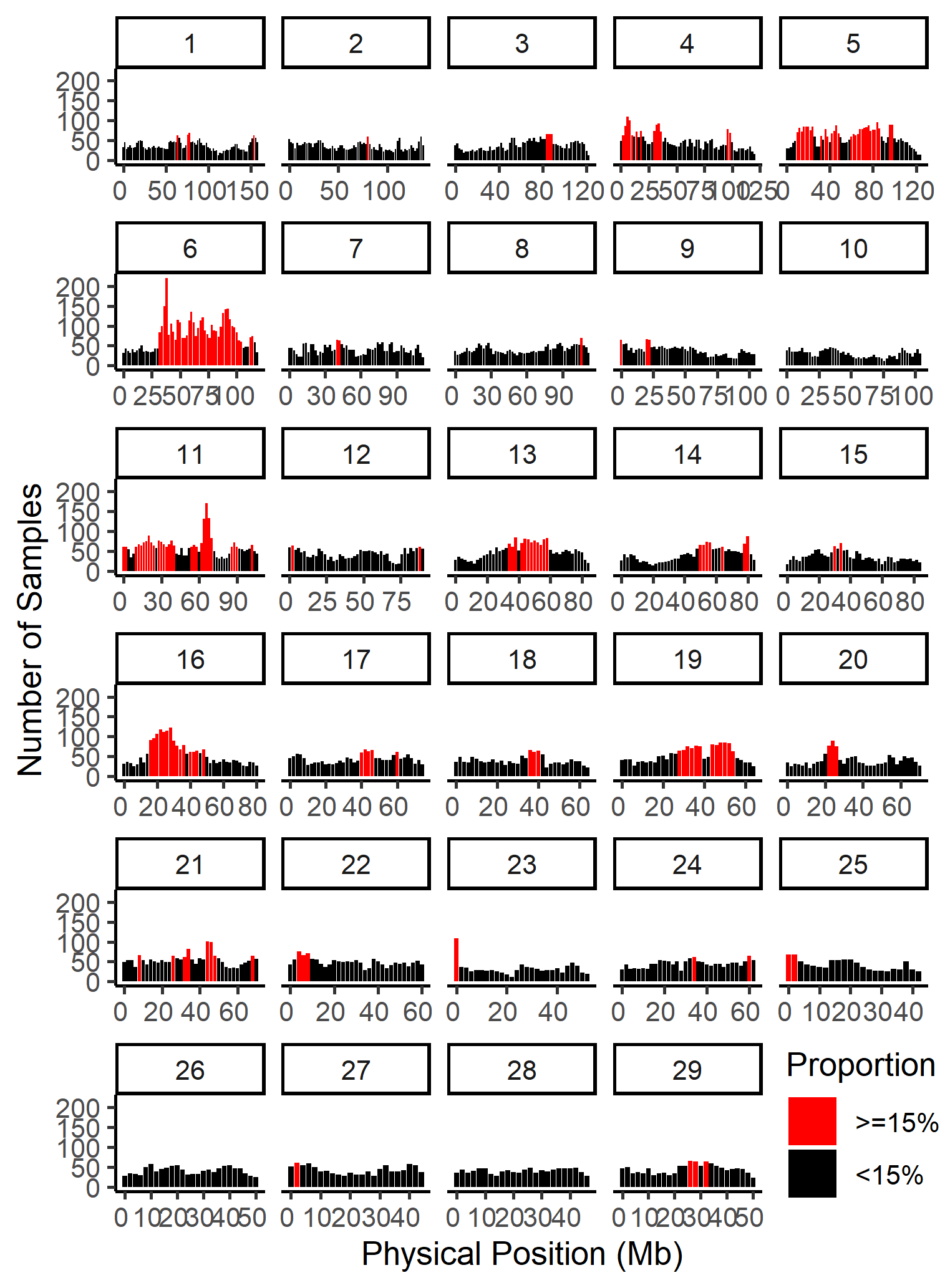
Figure.23 ROH Frequency Distribution
16. How do we visualise ROHs?
Visualising ROH is similar to visualising CNVs. The exception is that, because length is particularly informative for ROHs (about the age of inbreeding), the ROHs are coloured by their lengths. The roh_visual function can plot ROHs, either across the whole genome, or chromosome by chromosome. It also supports restricting plotting to regions of interest, and allows adding a panel of gene locations.
16.1 Plot ROH by Chromsome
To plot a single chromosome, use the chr_id argument.
roh_visual(clean_roh = "cnv_clean/cnvpart_roh.cnv",
           chr_id = 6,
           width_1 = 14,
           height_1 = 9,
           folder = "roh_visual",
           col_short = "red",
           col_mid = "blue",
           col_long = "black")
#> Preparing plot data...
#> Task done, plot was stored in working directory.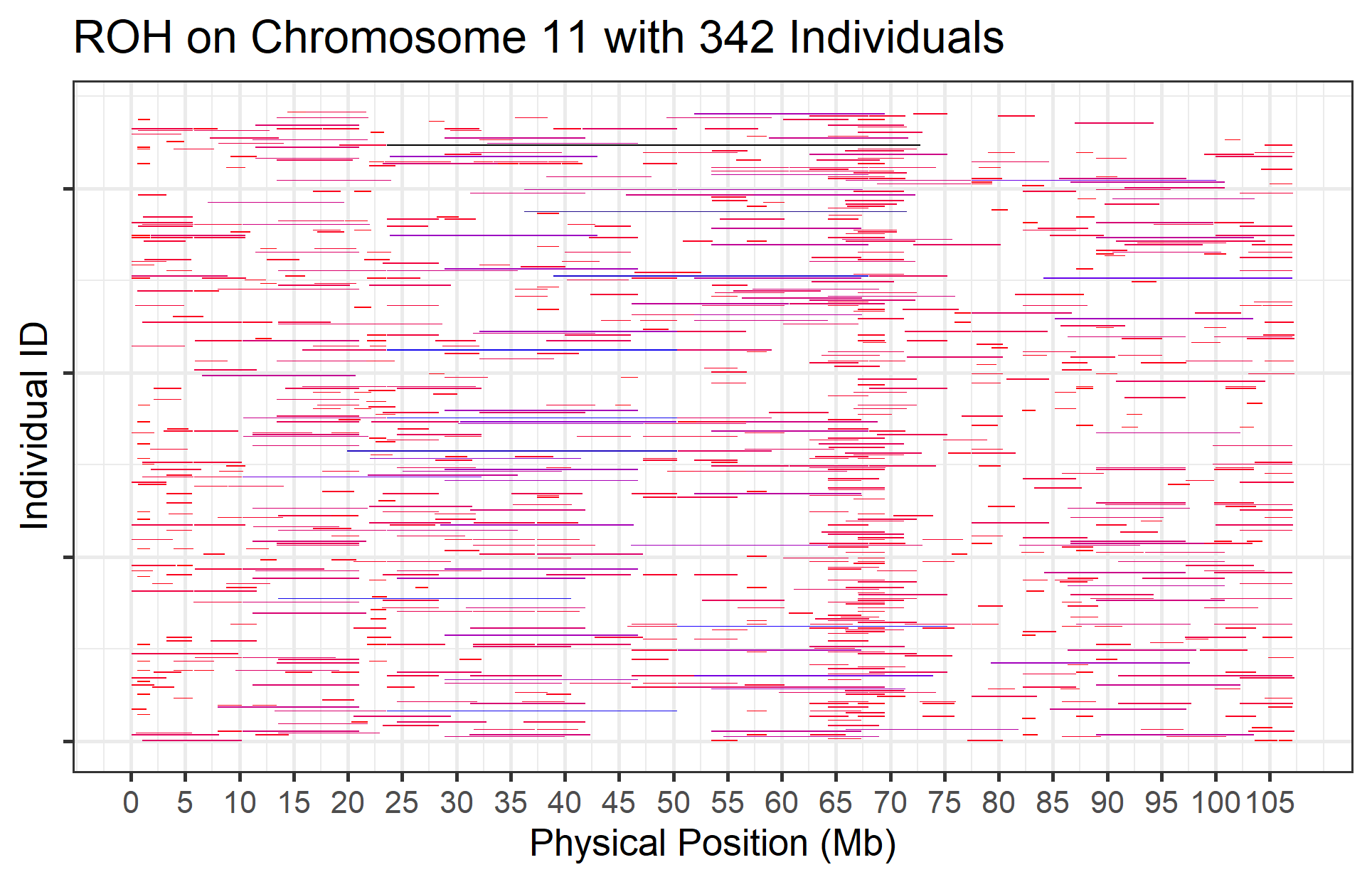
Figure.24 ROH on Chromosome 6
16.2 Plot ROH by single region
To plot a single region of interest, add the start_position and end_position arguments (units in megabases).
roh_visual(clean_roh = "cnv_clean/cnvpart_roh.cnv",
           chr_id = 6,
           start_position = 36.5,
           end_position = 40.6,
           width_1 = 16)
#> Preparing plot data...
#> [1] "Task done, plot was stored in working directory."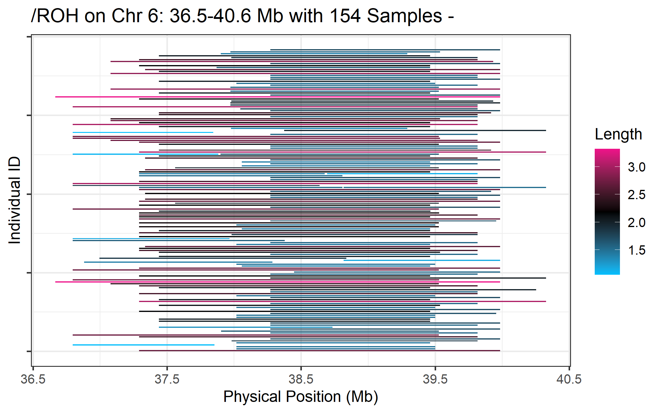
Figure.25 ROH on Chr6:35.0-42.5 Mb
16.3 How can we present annotated genes above the ROH plot?
To add a panel of gene locations, add the refgene argument, pointing to a file containing genes annotated on the appropriate reference genome.
roh_visual(clean_roh = "cnv_clean/cnvpart_roh.cnv",
           chr_id = 6,
           start_position = 36.5,
           end_position = 40.61,
           refgene = "refgene/cow_UMD_UCSC.txt")
#> Warning: Removed 2 rows containing missing values (geom_vline).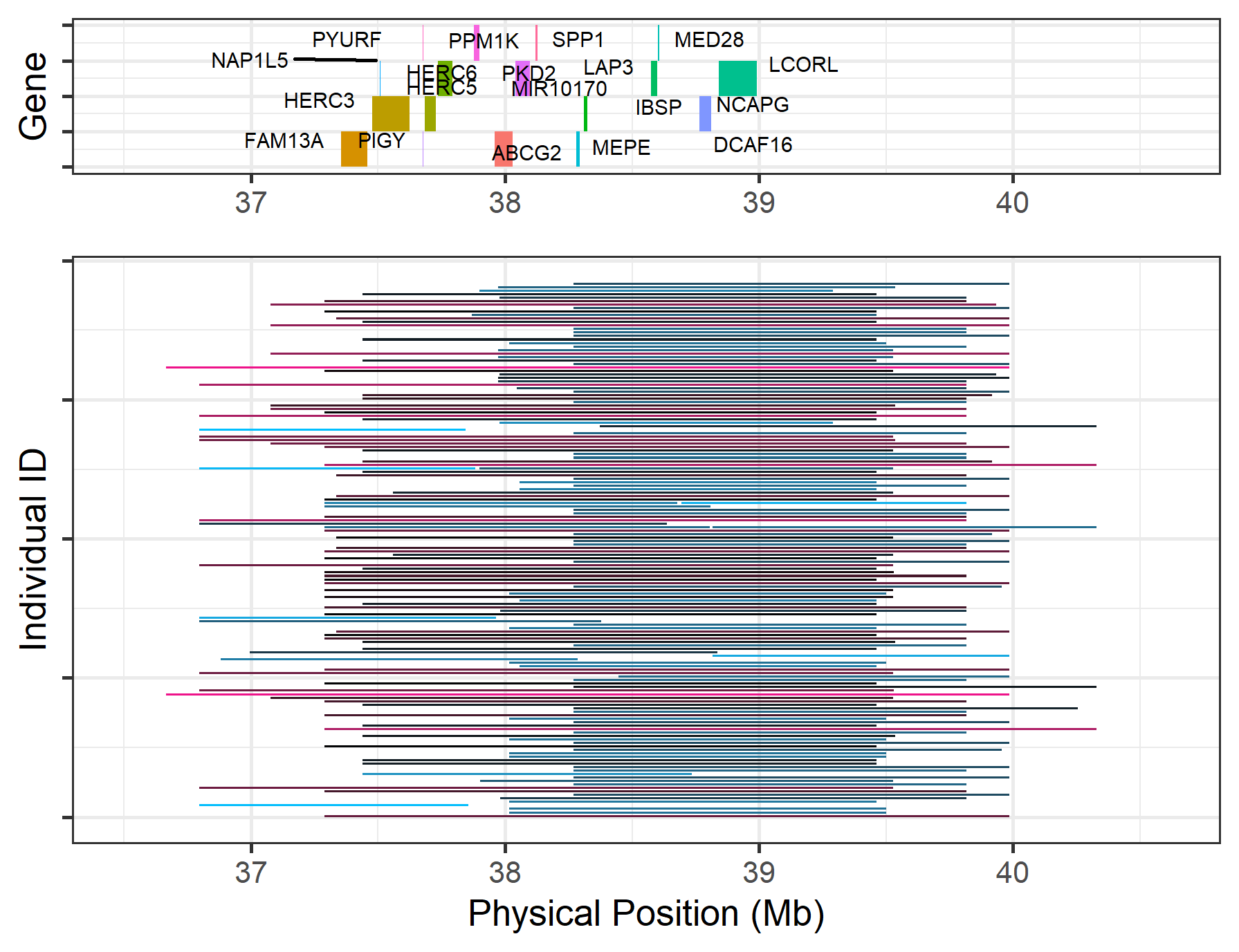
Figure.26 Annotation of ROH on Chr6:36.5-40.5
If the ROH region has too many genes, plotting all the gene names will make the figure look too busy. We can choose the most important region(s) to plot using the show_names argument. In this example, we set two regions with the following argument: show_name = c(37.28, 37.49, 38.25, 39.52). This will show the gene names in two regions: (37.28 - 37.49 Mb) and (38.25 - 39.52 Mb).
roh_visual(clean_roh = "cnv_clean/cnvpart_roh.cnv",
           chr_id = 6,
           start_position = 36.5,
           end_position = 40.5,
           refgene = "refgene/cow_UMD_UCSC.txt",
           show_name = c(37.28, 37.49, 38.25, 39.52), col_short = "black", col_mid = "green", col_long = "red")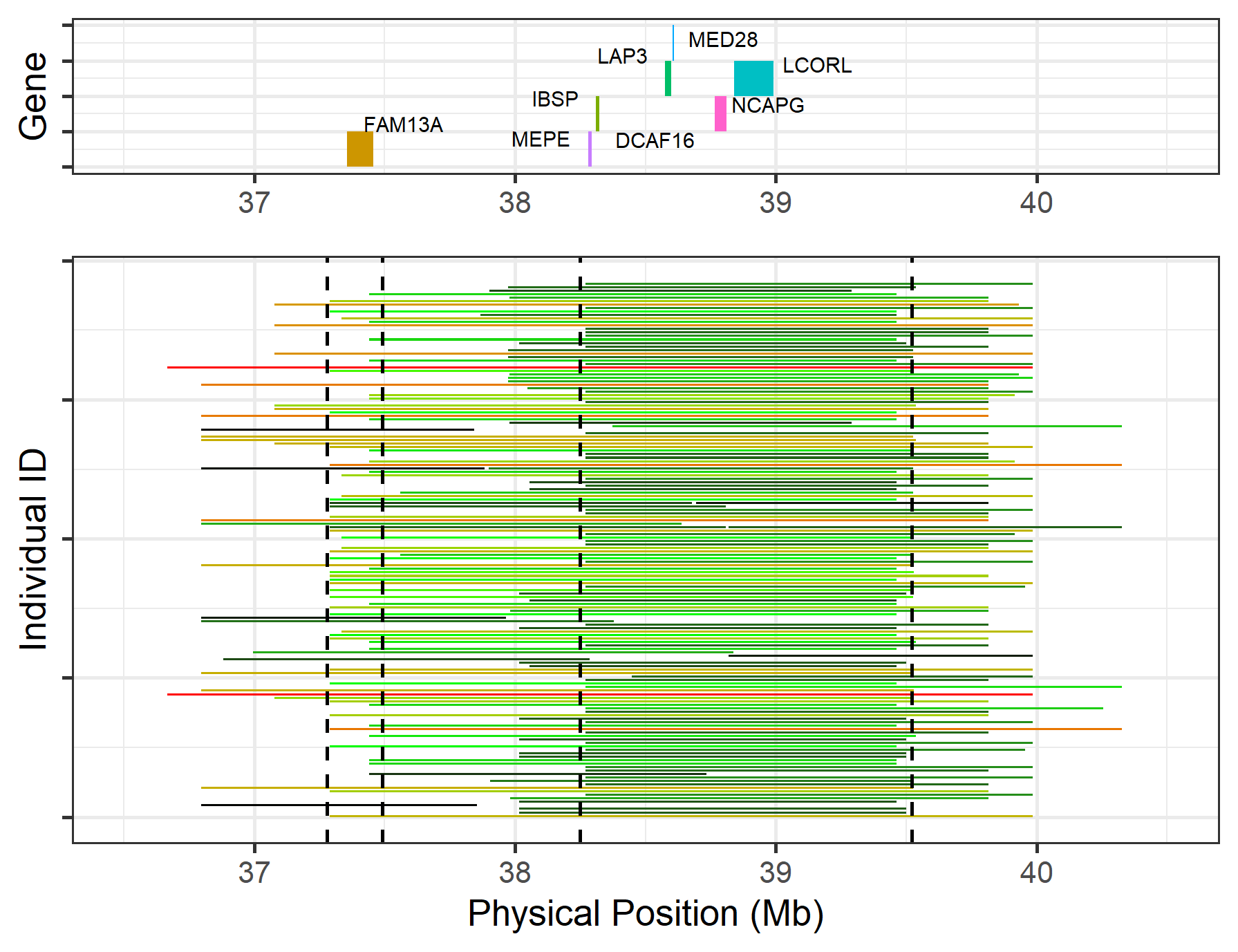
Figure.27 Customised gene annotations on Chr6:36.5-40.5 Mb
16.4 How do we plot the full length of ROH for all samples that had a ROH in a given region?
Above, We have plotted ROH in an interested region, but that method can only plot short ROHs which located in the given region, it will remove some longer ROHs which are partially overlapped to the given interval, that method can made a nice picture but will lost some samples, it still useful because we already know the sample size in that region. But if we want to present the whole length of ROH overlapped to our interested region (Such as a region of target gene), we can assign a vector to ‘target_region’ argument in ‘roh_visual’ function.
roh_visual(clean_roh = "cnv_clean/cnvpart_roh.cnv",
           target_region = c(6,38.25,39.52), #within the vector, the first integer indicate Chromosome. the rest are the start and end point, unit in megabases
           col_short = "red", #optional
           col_mid = "gold", #optional
           col_long = "blue", #optional
           height_1 = 12, #optional
           width_1 = 14)
#> Preparing plot data...
#> Task done, plot was stored in working directory.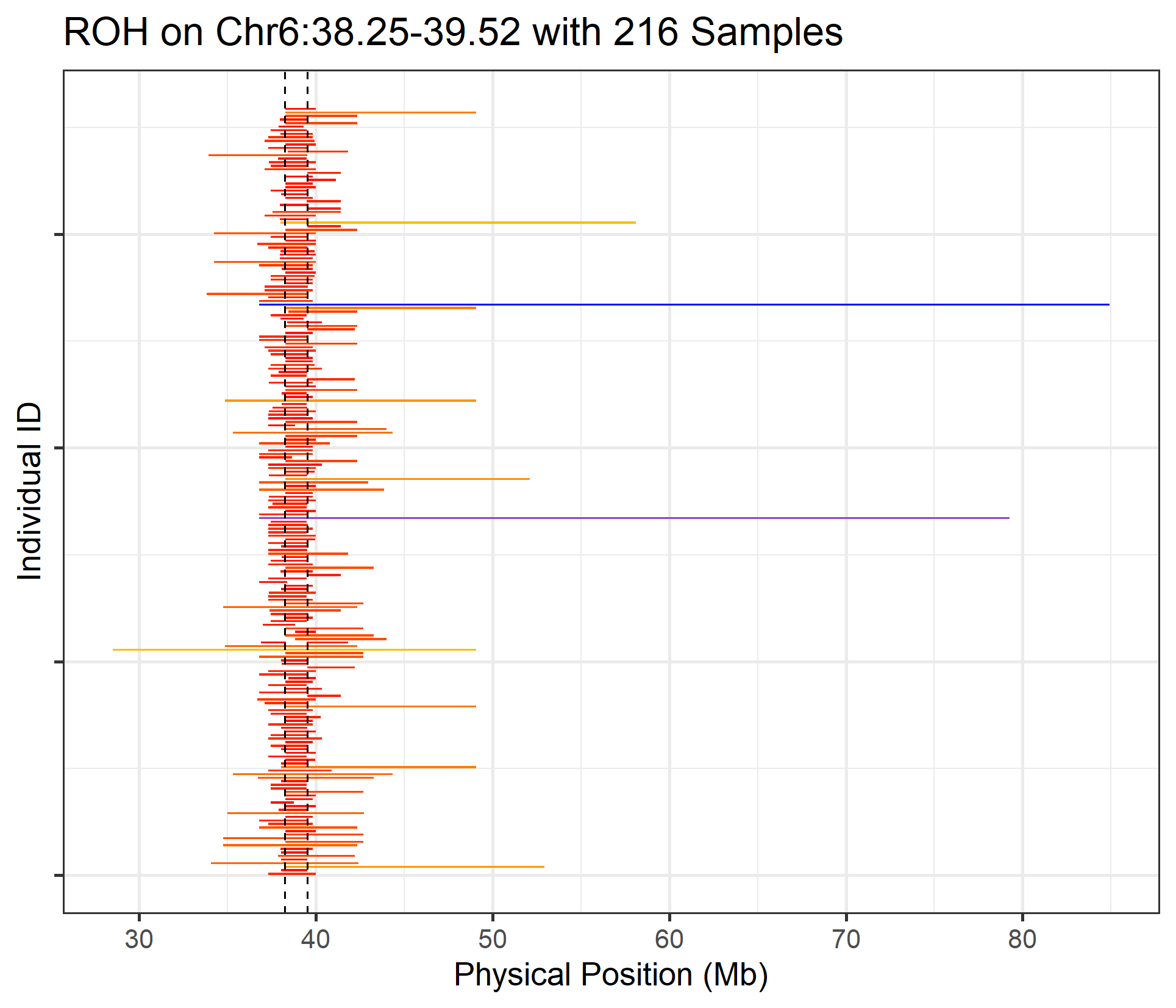
Figure.28 ROHs with full length on target region Chr6:38.25-39.52 Mb
16.5 How do we plot ROHs on an interested sample?
When we have some interested individuals, we can plot all the ROHs for these samples separately by setting the ‘individual_id’ arguments as following:
roh_visual(clean_roh = "cnv_clean/cnvpart_roh.cnv",
           individual_id = "201094560008_R04C01",
           height_1 = 14, #optional
           width_1 = 22,  #optional
           col_short = "green", #optional
           col_mid = "yellow", #optional
           col_long = "red")
#> Preparing plot data...
#> Task done, plot was stored in working directory.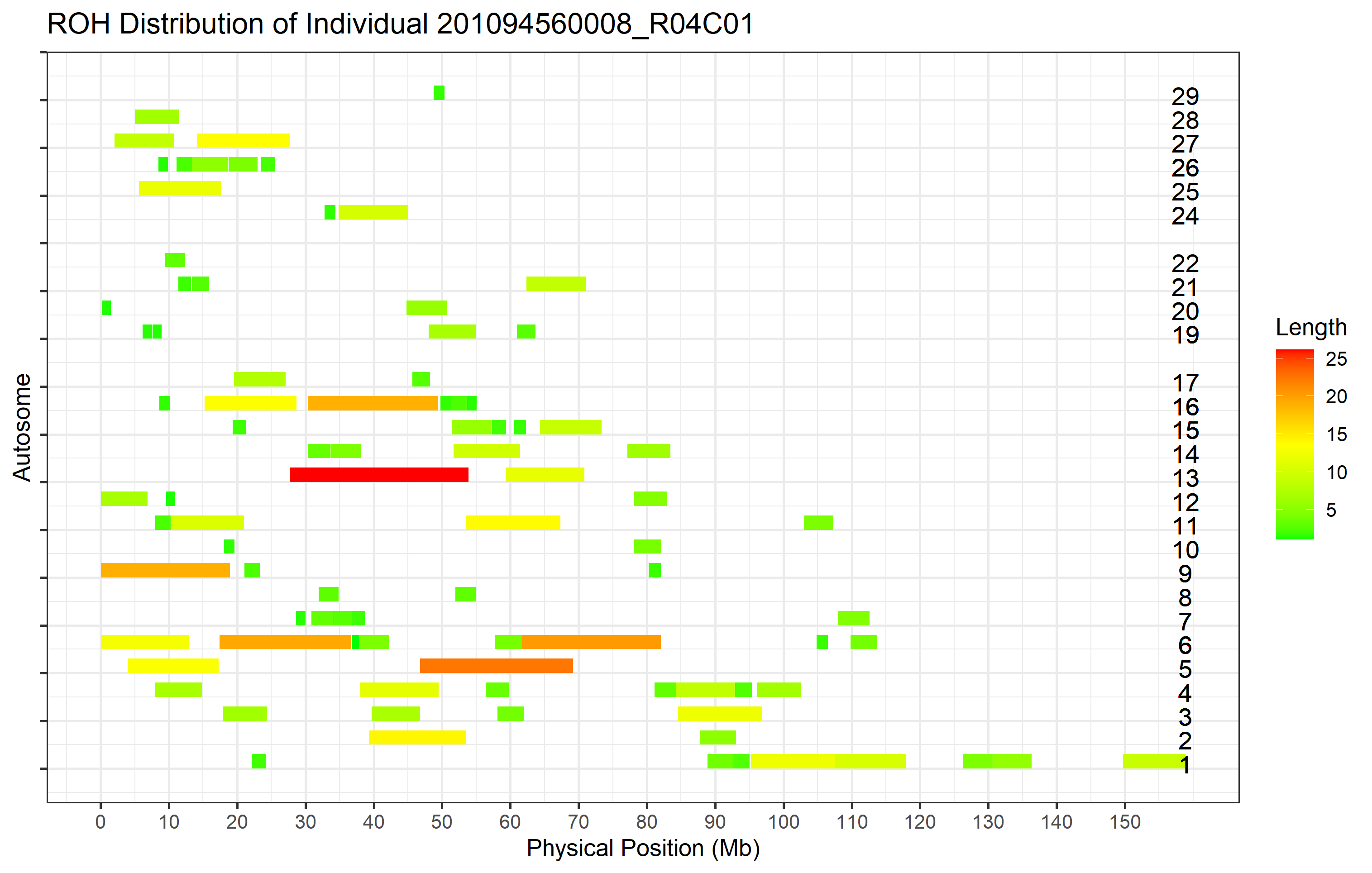
Figure 29. ROHs on interested Sample
17. How do we get haplotype for ROH region?
ROH results will return us some long regions, but we may interested on some specific genes in the ROH region that experienced strong selection. Get the haplotypes of these genes in our experimental population may help us to find out some interesting patterns. we known that the ROH region generated by SNPs may be discontinuous due to insufficient marker density, beside, when infer ROH we considered the influence of genotyping quality by setting the minimal window size, accepting some missing value or maximum heterozygosity SNPs in the window, these conditions will exclude the short ROH regions in the final results. For instance, when we get the haplotype for a short region (such as a Gene), the frequency of homozygosity haplotypes may differing to the original ROH region it located.
The ‘get_haplotype’ function can help us to get the haplotype for all samples by given region. But now the application is limited, it only accept the phased genotype by Beagle (Version 5.1) with physical position, we may expend the compatibility later if necessary. The standard format of phased genotype and demo data used at here can be download from our github repository (https://github.com/JH-Zhou/HandyCNV/tree/master/vignettes/orse_chr22_phased.vcf.gz). Now, let’s go ahead and make haplotypes.
Extracting the haplotype will take three steps and combine three functions. The first step is to prepare the standard format for ‘HandyCNV’. We can use ‘prepare_geno’ function to prepare the phased genotype. We can also assign the ‘convert_letter = TRUE’ in ‘pre_phased’ function to convert the format of haploids from 0,1 to letters. See code as following. After running, it will return three list files contain the map, genotype and the columns index file.
genotype_by_number <- prep_phased(phased_geno = "orse_chr22_phased.vcf.gz") #'orse_chr1_phased.vcf.gz' is the demo data, need to download and save it in working directory
#> Reading input file...
#> Spliting Sample columns...
#> Tansposing genotype...
genotype_by_letter <- prep_phased(phased_geno = "orse_chr22_phased.vcf.gz", convert_letter = T) #'orse_chr1_phased.vcf.gz' is the demo data, need to download and save it in your working
#> Reading input file...
#> Coverting haplotype from 0, 1 to Ref and ALT...
#> Spliting Sample columns...
#> Tansposing genotype...
Second step, we need to assign the interested region. Here we take the GDF5 gene as example, it located on Chr22:26,183,610-26,188,173 bp. The idea in this step is to find out the closest SNPs in this SNP chip.
region <- closer_snp(phased_input = genotype_by_letter$map, #the map file in the list generated in 'pre_phased' function above
                     chr = 22, start = 43.771500, end = 43.856076) #physical position unit in 'megabases'
#> # A tibble: 1 x 2
#>        min      max
#>      <int>    <int>
#> 1 43778695 43849927
Third step to get haplotype. It will return two lists contains the reocding haplotype and the index of recode type and the original haploid.
haplotype_number <- get_haplotype(geno = genotype_by_number, pos = region)
#> [1] 10421
#> [1] 10440
#> There are 20 SNPs in this region...
#> Recoding Haploid...
#> Generating Haplotype...
haplotype_letter <- get_haplotype(geno = genotype_by_letter, pos = region)
#> [1] 10421
#> [1] 10440
#> There are 20 SNPs in this region...
#> Recoding Haploid...
#> Generating Haplotype...
Now, we can count the frequency of each haplotype in our population and to check what the haploids are in these haplotypes.
data.frame(table(haplotype_number$hap_type$Recode_Type, dnn = "Haplotype"))
#>    Haplotype Freq
#> 1        1-1  156
#> 2       1-17    1
#> 3       1-18    1
#> 4        1-2   57
#> 5       1-22    1
#> 6       1-23    1
#> 7       1-26    1
#> 8        1-3   21
#> 9       1-30    1
#> 10      1-31    1
#> 11      1-34    1
#> 12      1-35    1
#> 13       1-4    8
#> 14       1-5    2
#> 15       1-6    1
#> 16     11-24    1
#> 17     12-20    1
#> 18     13-15    1
#> 19     19-25    1
#> 20      2-14    1
#> 21      2-28    1
#> 22       2-3    7
#> 23      2-32    1
#> 24       2-4    5
#> 25       2-7    2
#> 26       2-8    1
#> 27       2-9    1
#> 28     21-27    1
#> 29       3-4    1
#> 30       3-5    1
#> 31       3-6    1
#> 32      4-10    1
#> 33      4-29    1
#> 34      8-16    1
#> 35      9-33    1
haplotype_number$hap_index
#> # A tibble: 35 x 3
#>    Haploid               Freq Re_code
#>    <chr>                <int>   <dbl>
#>  1 00000000000000000000   410       1
#>  2 00000000000000001000    76       2
#>  3 10000000000000000000    31       3
#>  4 01001111110001100000    16       4
#>  5 00000000010000000000     3       5
#>  6 00000000000100000000     2       6
#>  7 00001001000000000000     2       7
#>  8 00001010000100000000     2       8
#>  9 01100111001001100000     2       9
#> 10 00000000000000000010     1      10
#> # ... with 25 more rows
data.frame(table(haplotype_letter$hap_type$Recode_Type, dnn = "Haplotype"))
#>    Haplotype Freq
#> 1        1-1  156
#> 2       1-11    1
#> 3       1-13    1
#> 4       1-14    1
#> 5       1-17    1
#> 6        1-2   57
#> 7       1-26    1
#> 8       1-29    1
#> 9        1-3   21
#> 10      1-30    1
#> 11      1-31    1
#> 12      1-33    1
#> 13       1-4    8
#> 14       1-5    2
#> 15       1-8    1
#> 16     15-25    1
#> 17     16-28    1
#> 18     18-35    1
#> 19      2-12    1
#> 20      2-21    1
#> 21       2-3    7
#> 22      2-34    1
#> 23       2-4    5
#> 24       2-6    1
#> 25       2-7    2
#> 26       2-9    1
#> 27     20-24    1
#> 28     22-27    1
#> 29       3-4    1
#> 30       3-5    1
#> 31       3-8    1
#> 32      4-23    1
#> 33      4-32    1
#> 34      6-19    1
#> 35      9-10    1
haplotype_letter$hap_index
#> # A tibble: 35 x 3
#>    Haploid               Freq Re_code
#>    <chr>                <int>   <dbl>
#>  1 TCCCTAGTTGCGTAAGTTTA   410       1
#>  2 TCCCTAGTTGCGTAAGCTTA    76       2
#>  3 CCCCTAGTTGCGTAAGTTTA    31       3
#>  4 TTCCCGACCTCGTCGGTTTA    16       4
#>  5 TCCCTAGTTTCGTAAGTTTA     3       5
#>  6 TCCCCAATTGCATAAGTTTA     2       6
#>  7 TCCCCAGCTGCGTAAGTTTA     2       7
#>  8 TCCCTAGTTGCATAAGTTTA     2       8
#>  9 TTTCTGACTGAGTCGGTTTA     2       9
#> 10 CCCCTAACTGAGTAAGTTTA     1      10
#> # ... with 25 more rows
Then, visualize haplotype of BMP7 gene.
haplo_visual(haplotype = haplotype_letter, xlab_text = "BMP7 Gene ")

18. How do we convert coordinates for CNV, CNVR, ROH, or any other intervals?
The function convert_coord can used to convert coordinates for lists of intervals. Currently, the function is limited to inputs generated by the convert_map function, and can only convert the coordinates for intervals on the same type of SNP Chip. Converting coordinates may change the total length of the intervals, as of the positions and orders of the SNPs on the chromosome will potentially differ between various versions of reference genome; therefore, we should pay attention to the quality of the conversion, and use the results with caution. The function produces a summary table that summarises how many intervals were converted successfully, and reports on the differences in length between the converted and original intervals.
The proxy_range argument supports adjusting the genomic range to search and assign “proxy” locations for markers which are missing in the target map, in order to try to best reduce the loss of intervals after conversion. The principal is try to reduce the length of the intervals that were assigned to the proxy locations. For missing markers at the start positions, the search will begin at the missing position and proceed downsteam, selecting the closest suitable marker as the proxy position. For the end position, the search will begin from the missing end interval and proceed upsteam, again assigning the closest suitable marker as the proxy position. If no suitable markers can be found within proxy_range basepairs, the interval will be classed at “Missing”.
The optional argument len_diff_threshold is a quality control measure on the newly converted intervals that imposes a maximum difference of length between converted and original intervals. Only intervals with remapped positions within len_diff_threshold basepairs of the original position will pass the threshold.
Here, we convert the CNVPartition CNVR results from UMD3.1 coordinates to ARS1.2. The outputs are saved into the convert_coord_penn_cnv folder, and summary statistics about the conversion are displayed below.
convert_coord(input_def = "cnv_clean/cleancnv.cnv",
              def_tar_map = "convert_map/def_tar_map.map",
              proxy_range = 100000,
              len_diff_threshold = 100000,
              folder = "convert_coord_penn_cnv")
#> [1] "'def_tar_map' file passed input check..."
#> [1] "The quality check of converion on Start Position as below: FALSE means not match between two version."
#>
#>    Match Mismatch
#>     4396      180
#> [1] "The quality check of converion on End Position as below: FALSE means not match between two version."
#>
#>    Match Mismatch
#>     4322      254
#> [1] "4104 Intervals passed quality check."
#>
#> Fail Pass
#>  472 4104
#>                                  Item    Length Number
#> 1                      Total Original 974963676   4576
#> 2                   Succeed Original  891042504   4104
#> 3                  Succeed Convertion 897762659      -
#> 4                   Failed convertion  77201017    472
#> 5 Difference Converted minus Original  -6720155      -
We can also convert coordinates from the target map to the default map. For example, let’s convert the PennCNV ARS results to UMD 3.1. After converting the coordinates of CNVs or CNVRs, we could use the results which passed the quality check to make comparisons with the compare_cnv and compare_cnvr functions as section 8 and 9 described.
convert_coord(input_def = "call_cnvr_standard/cnvr.txt",
              proxy_range = 100000,
              len_diff_threshold = 100000,
              def_tar_map = "convert_map/def_tar_map.map",
              folder = "convert_coord_penn_cnvR")
#> [1] "'def_tar_map' file passed input check..."
#> [1] "The quality check of converion on Start Position as below: FALSE means not match between two version."
#>
#>    Match Mismatch
#>      871       10
#> [1] "The quality check of converion on End Position as below: FALSE means not match between two version."
#>
#>    Match Mismatch
#>      870       11
#> [1] "835 Intervals passed quality check."
#>
#> Fail Pass
#>   46  835
#>                                  Item    Length Number
#> 1                      Total Original 286942723    881
#> 2                   Succeed Original  270103909    835
#> 3                  Succeed Convertion 271977583      -
#> 4                   Failed convertion  14965140     46
#> 5 Difference Converted minus Original  -1873674      -
19. How do we make a fast SNP density plot from Plink map file?
Plotting SNP density may help us learn about the SNP distribution on chromosomes. The parameter of SNP density may affect ROH detection in some tools. ‘plot_snp_density’ only working with map file that has four columns in the order as follows: Chromosome, SNP ID, Position in Morgans, Physical Position. No header required.
plot_snp_density(map = "convert_map/target_plink.map",
                 max_chr = 24, #optional
                 top_density = 60, #optional
                 low_density = 20, #optional
                 color_top = "red", #optional
                 color_low = "blue", #optional
                 color_mid = "black", #optional
                 legend_position = c(0.9, 0.1), #optional
                 x_label = "Physical position\n<U+7269><U+7406><U+4F4D><U+7F6E>"NA#optionalNA= "SNPs/Mb\n<U+6BCF>1Mb<U+533A><U+95F4><U+7684>SNP<U+6570>"NA#optionalNA= 5)
#> The total number of SNPs on selected chromosomes are 119249
#> The number of regions on different SNP density groups as following:
#>
#>  <=20  >=60 20-60
#>    39   397  1849
#> The Mean of SNPs density is  52  SNPs/Mb
#> The Mean + SD of SNP density is  73  SNPs/Mb
#> The Mean - SD of one SD is  31  SNPs/Mb
#save the plot by 'ggsave'
#ggsave(filename = "snp_density.png", width = 26, height = 18, units = "cm", dpi = 350)
Figure 31. SNP density distribution